The bundled datasets
Four small, pre-cleaned planning datasets travel with the package rather than being downloaded. That matters more than it looks: a problem set built on a live URL stops working the month a city reorganises its open-data portal, and a class that spends its first twenty minutes on data wrangling never gets to the statistics.
They are also real — extracts of public data, cleaned but not invented — so the numbers a student reports are numbers about an actual place.
import bayesplain as bp

print(bp.datasets.describe())
collisions       12,000 rows   Traffic collisions in Los Angeles and San Diego counties, 2019-2023, one row per collision.
la_blockgroups    5,361 rows   The same ACS variables as la_tracts, for Los Angeles County block groups — a finer geography over identical ground.
la_tracts         2,412 rows   American Community Survey estimates for Los Angeles County census tracts, 2021.
parcels           7,869 rows   Residential parcels in Baltimore with assessed values, size, age, and construction type.
print(bp.datasets.describe("collisions"))
collisions  (12,000 rows)

Traffic collisions in Los Angeles and San Diego counties, 2019-2023, one row per collision.

Source: California SWITRS, via github.com/oturns/example_datasets; a random sample of collisions falling inside either county.

Columns
-------
  county            Los Angeles or San Diego
  year              year of the collision
  severity          fatal, severe injury, other injury, complaint of pain, or property damage only
  road_surface      dry, wet, snowy or icy, slippery
  alcohol_involved  whether alcohol was recorded as involved
  pedestrian        whether a pedestrian was involved
  bicycle           whether a bicycle was involved
  hit_and_run       whether the collision was a hit and run
  injured           number of people injured
  killed            number of people killed

Good for
--------
  - proportion — the share of collisions involving alcohol
  - compare_proportions — alcohol involvement in the two counties, which is the two-group comparison the course pivots on
  - contingency — severity against road surface
  - compare_means — people injured per collision, by county
  - compare_rates — people killed per 1,000 collisions, by county
  - categories — each county's share of collisions against its share of population
Collisions: the two-group comparison
df = bp.datasets.load_collisions()
counts = df.groupby("county").alcohol_involved.agg(["sum", "size"])
counts
| sum | size | |
|---|---|---|
| county | ||
| Los Angeles | 803 | 9886 |
| San Diego | 243 | 2114 |
res = bp.compare_proportions(
    counts["sum"].to_numpy(), counts["size"].to_numpy(),
    labels=list(counts.index),
)
res.sentence()
'San Diego is higher than Los Angeles with 100% probability; the best estimate of the gap is 3.4 percentage points, and the data are consistent with anything from 1.9 to 4.9 percentage points (95% credible interval).'
And a contingency table from the same file:
import pandas as pd

table = pd.crosstab(df.road_surface, df.severity)
table
| severity | complaint of pain | fatal | other injury | property damage only | severe injury |
|---|---|---|---|---|---|
| road_surface | |||||
| dry | 2246 | 63 | 1308 | 7235 | 304 |
| slippery | 5 | 0 | 5 | 15 | 1 |
| snowy or icy | 1 | 0 | 3 | 8 | 0 |
| wet | 196 | 7 | 95 | 489 | 19 |
print(bp.contingency(table).summary())
==========================================================================
 strength of association (Cramér's V) between rows and columns
==========================================================================

 BAYESIAN — what the data say about the quantity itself

   best estimate (median)    0.035
   95% credible interval     0.018 to 0.062  (HDI)
   P(above 0.100)            0.001

   Read: The best estimate of the association strength is 0.035, and the
         data are consistent with anything from 0.018 to 0.062 (95%
         credible interval).

 FREQUENTIST — Pearson chi-square test of independence

   chi-square (12 df)        14.84
   p-value                   0.2504  (not significant at 0.05)

   Read: If rows and columns were unrelated, data at least this extreme
         would turn up 25.0% of the time.

   --------------------------------------------------------------------

   How they line up
     Neither one finds much. The test cannot rule out that rows and
     columns were unrelated (p = 0.25), and the posterior puts the
     effect somewhere in 0.018 to 0.062, measured against a 0.100 bar
     for a small effect. Note that these are different questions with a
     common answer here, not one question asked twice: the interval is
     the more useful of the two, because it is wide enough to show you
     which conclusions the data cannot yet separate.

--------------------------------------------------------------------------
 assumption   prior: uninformed — Dirichlet(1)
 precision    100,000 independent draws; Monte Carlo error on the mean
              is ±3.7e-05. These are exact samples, not a Markov chain.
 note         8 of 20 cells have expected counts below 5, where the chi-
              square approximation is unreliable. The posterior is
              unaffected — it just gets wider, which is the honest
              response to thin data.
 note         Cramér's V cannot be negative, so P(above 0.1) is measured
              against a conventional 'small association' bar rather than a
              null. Set threshold= to a value that matters for your
              decision instead.
 next         .probability('>', x)  .decide(rope=(lo, hi))  .sensitivity()
==========================================================================
Tracts and block groups: the same place, twice
This pair exists for one purpose. Identical variables, identical county, two aggregations — and a different answer.
tracts = bp.datasets.load_tracts().dropna(subset=["median_income", "median_rent"])
blocks = bp.datasets.load_blockgroups().dropna(subset=["median_income", "median_rent"])

for name, d in [("tracts", tracts), ("block groups", blocks)]:
    res = bp.correlation(
        d.median_income, d.median_rent,
        labels=["median income", "median rent"], aggregated=True,
    )
    lo, hi = res.interval()
    print(f"{name:13} n={len(d):5}  r={res.point():.3f}  95% CI [{lo:.3f}, {hi:.3f}]")
tracts        n= 2412  r=0.781  95% CI [0.765, 0.796]
block groups  n= 5361  r=0.695  95% CI [0.681, 0.709]
The intervals do not overlap. This is not sampling noise that more data would settle — it is the modifiable areal unit problem, and it means the correlation is partly a property of the boundaries someone drew. Redraw them and the number moves.
The related warning is ecological correlation: a relationship between area
averages can differ from the relationship among individuals, sometimes in sign.
Passing aggregated=True attaches both caveats to the result, so they travel
with the analysis rather than living only in a lecture.
res = bp.correlation(
    tracts.median_income, tracts.median_rent, aggregated=True
)
for note in res.notes:
    print("-", note)
- A correlation is not a cause. Nothing in this analysis rules out a third variable driving both, or the arrow pointing the other way.
- These rows are areas, not people. A correlation between area averages can differ from the correlation among individuals, sometimes in sign (Robinson 1950), and it will change if the boundaries are redrawn. Report the geography you used.
Parcels: groups, and why the smallest one lies
parcels = bp.datasets.load_parcels()
parcels.groupby("construction").assessed_value.agg(["count", "median"])
| count | median | |
|---|---|---|
| construction | ||
| Brick | 5802 | 120700.0 |
| Frame | 669 | 139700.0 |
| Shingle Asbestos | 287 | 146000.0 |
| Shingle Wood | 140 | 192100.0 |
| Siding | 829 | 160900.0 |
| Stucco | 142 | 187700.0 |
groups = {
    name: sub.assessed_value.to_numpy()
    for name, sub in parcels.groupby("construction")
}

raw = bp.compare_groups(groups, unit="dollars")
pooled = bp.compare_groups(groups, unit="dollars", pool=True)
import numpy as np

comparison = pd.DataFrame({
    "n": [len(groups[g]) for g in raw.group_names],
    "unpooled": [np.median(raw.group_draws[g]) for g in raw.group_names],
    "pooled": [np.median(pooled.group_draws[g]) for g in raw.group_names],
    "weight": pooled.pooling["weights"],
}, index=raw.group_names).round(2)
comparison.sort_values("n")
| n | unpooled | pooled | weight | |
|---|---|---|---|---|
| Shingle Wood | 140 | 251347.46 | 232075.03 | 0.70 |
| Stucco | 142 | 251650.66 | 231502.08 | 0.69 |
| Shingle Asbestos | 287 | 148597.56 | 149403.87 | 0.98 |
| Frame | 669 | 160267.37 | 161175.84 | 0.97 |
| Siding | 829 | 193271.77 | 193117.25 | 0.97 |
| Brick | 5802 | 157090.10 | 157248.61 | 1.00 |
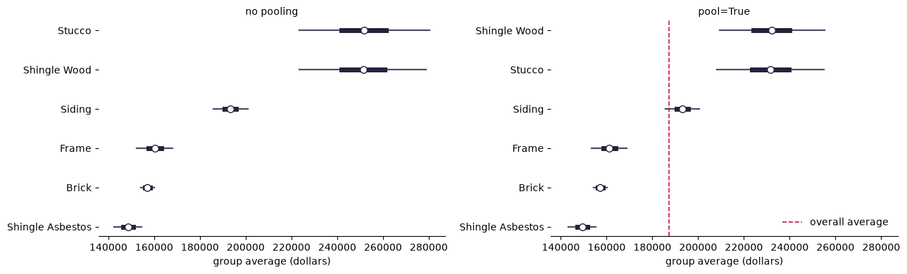
The groups with the fewest parcels have the smallest weights, meaning they were pulled hardest toward the overall average. That is the correction working: a small group has room to wander, and its observed average is weaker evidence about its true value than a large group’s is.
import matplotlib.pyplot as plt

fig, axes = plt.subplots(1, 2, figsize=(13, 4), sharex=True)
raw.plot(kind="forest", ax=axes[0])
axes[0].set_title("no pooling", fontsize=10)
pooled.plot(kind="forest", ax=axes[1])
axes[1].set_title("pool=True", fontsize=10)
fig.tight_layout()
Provenance
Every dataset records where it came from:
for name in bp.datasets.available():
    print(f"{name}: {bp.datasets.DATASETS[name].source}\n")
collisions: California SWITRS, via github.com/oturns/example_datasets; a random sample of collisions falling inside either county.

la_blockgroups: ACS 5-year estimates, via github.com/oturns/example_datasets.

la_tracts: ACS 5-year estimates, via github.com/oturns/example_datasets.

parcels: Maryland PropertyView assessor records, via github.com/oturns/example_datasets; residential parcels only, with implausible sizes and values trimmed.