Quickstart
Every analysis in bayesplain returns the same object with the same methods,
so what you learn here works for all of them.
import bayesplain as bp

bp.__version__
'0.1.1.dev10+g676e1d899'
One analysis, both frameworks
Two counties’ rates of alcohol involvement in traffic collisions, from the bundled data.
df = bp.datasets.load_collisions()
counts = df.groupby("county").alcohol_involved.agg(["sum", "size"])
counts
| sum | size | |
|---|---|---|
| county | ||
| Los Angeles | 803 | 9886 |
| San Diego | 243 | 2114 |
res = bp.compare_proportions(
    successes=counts["sum"].to_numpy(),
    n=counts["size"].to_numpy(),
    labels=list(counts.index),
)
print(res.summary())
==========================================================================
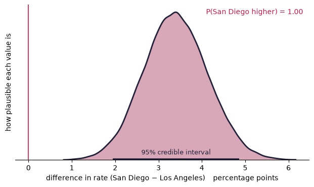
 difference in rate (San Diego − Los Angeles)
==========================================================================

 BAYESIAN — what the data say about the quantity itself

   best estimate (median)    3.4 percentage points
   95% credible interval     1.9 to 4.9 percentage points  (HDI)
   P(San Diego higher)       1.000

   Read: San Diego is higher than Los Angeles with 100% probability; the
         best estimate of the gap is 3.4 percentage points, and the data
         are consistent with anything from 1.9 to 4.9 percentage points
         (95% credible interval).

 FREQUENTIST — two-proportion z-test (equivalently chi-square, 1 df)

   chi-square (1 df)         24.89
   p-value                   6.069e-07  (significant at 0.05)
   95% confidence interval   1.9 to 4.8 percentage points  (Wald)

   Read: If the two rates were identical, data at least this extreme would
         turn up less than once in a million studies.

   --------------------------------------------------------------------

   How they line up
     Both point the same way here, so the choice between them is not
     about the conclusion but about what you can say. 'Significant'
     licenses a claim about the data; the posterior licenses a claim
     about the size of the effect, which is what a recommendation
     actually needs.

--------------------------------------------------------------------------
 assumption   prior: uninformed — Beta(1, 1)
 precision    100,000 independent draws; Monte Carlo error on the mean
              is ±2.4e-05. These are exact samples, not a Markov chain.
 next         .probability('>', x)  .decide(rope=(lo, hi))  .sensitivity()
==========================================================================
The posterior comes first because it is what a recommendation is written from. The conventional test comes second because you will meet it in every report you read, and because seeing both is the only reliable way to learn what each one actually claims.
Asking a question the p-value cannot answer
res.probability(">", 0.02) # P(the gap exceeds 2 percentage points)
0.97199
print(res.decide(rope=(-0.01, 0.01)))
PRACTICALLY DIFFERENT — the whole 95% credible interval sits outside the
                        range you called too small to act on (−1.0 to 1.0
                        percentage points), so the difference is both real
                        and big enough to matter
A “ROPE” is a region of practical equivalence: a range you decided in advance is too small to act on. Comparing the credible interval against it replaces “reject the null” with a rule that refers to consequences.
The memo sentence
res.sentence()
'San Diego is higher than Los Angeles with 100% probability; the best estimate of the gap is 3.4 percentage points, and the data are consistent with anything from 1.9 to 4.9 percentage points (95% credible interval).'
Have students write this themselves before revealing the method. Otherwise the convenience quietly becomes the learning objective.
Translating between frameworks
print(res.translate())
THE QUANTITY: difference in rate (San Diego − Los Angeles)

What the posterior says
  Given this data and the stated prior, there is a 95% probability the
  value lies in the range 1.9 to 4.9 percentage points, and a 100%
  probability it is greater than zero. Both are statements about the
  quantity itself.

What the two-proportion z-test (equivalently chi-square, 1 df) says
  If the two rates were identical, data at least this extreme would turn
  up less than once in a million studies.
  It is not the probability that the null is true, not the probability
  this finding is wrong, and it says nothing about how large the effect
  is. p = 6.1e-07 is a statement about data given a hypothesis, not about
  a hypothesis given data.
  Across many repetitions of this study, 95% of intervals built this way
  would contain the true value. It does not say there is a 95% chance the
  true value lies in the range 1.9 to 4.8 percentage points — that
  sentence is only available for a credible interval.

How they line up
  Both point the same way here, so the choice between them is not
  about the conclusion but about what you can say. 'Significant'
  licenses a claim about the data; the posterior licenses a claim
  about the size of the effect, which is what a recommendation
  actually needs.
How much does the prior matter?
print(res.sensitivity())
HOW MUCH DOES THE PRIOR MATTER?
quantity: difference in rate (San Diego − Los Angeles)
interval in percentage points

prior                         95% interval            P(dir)        BF10
--------------------------------------------------------------------------
uninformed — Beta(1, 1)       1.9 to 4.9               1.000    2.11e+03
jeffreys — Beta(0.5, 0.5)     1.9 to 4.8               1.000    2.17e+03
gentle — Beta(2, 2)           2.0 to 4.9               1.000    1.21e+03
skeptical — Beta(10, 10)      2.2 to 5.1               1.000        1.45

Verdict: the estimate barely moves. The direction probability shifts by
         less than 0.05 across every assumption tried and the interval
         width by less than 1%, so this conclusion is driven by the data.
         Report it, and note that you checked.

But note: the Bayes factor is a different story: it moves by a factor of
          1497 over the same priors, while the interval hardly budged.
          That gap is not a bug in either number — it is why this package
          leads with the estimate. Locating a value is a question the data
          can mostly answer on its own; grading the evidence for one model
          against another cannot be separated from what you assumed the
          alternative looked like.
Notice what this usually shows: the credible interval barely moves across every prior, while the Bayes factor moves a great deal. They are answering different questions, and that asymmetry is why this package leads with the estimate.
Seeing it
res.plot();
res.plot(kind="components");
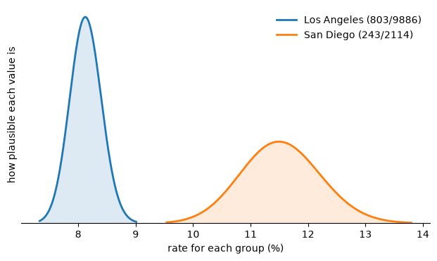
The second plot is the one that explains where a difference came from.
res.plot_kinds()
['posterior', 'prior_posterior', 'components']
The Bayes factor, when someone asks
print(res.bayes_factor())
BF10 = 2.11e+03  (extreme evidence for a difference)
BF01 = 0.000475
Compares 'the two groups have different rates' against 'they have the same rate', under a flat Dirichlet prior over the 2x2 table. Prior-sensitive; run .sensitivity() before quoting it.
Deliberately a method call rather than part of the summary.
The other analyses
parcels = bp.datasets.load_parcels()

rowhouses = parcels.loc[parcels.rowhouse, "assessed_value"]
detached = parcels.loc[~parcels.rowhouse, "assessed_value"]

means = bp.compare_means(
    rowhouses, detached,
    labels=["rowhouse", "detached"], unit="dollars",
)
means.sentence()
'detached is higher than rowhouse with 100% probability; the best estimate of the gap is 9362.39 dollars, and the data are consistent with anything from 3051.65 to 15752.44 dollars (95% credible interval).'
groups = {
    name: sub.assessed_value.to_numpy()
    for name, sub in parcels.groupby("construction")
}
res_groups = bp.compare_groups(groups, unit="dollars", pool=True)
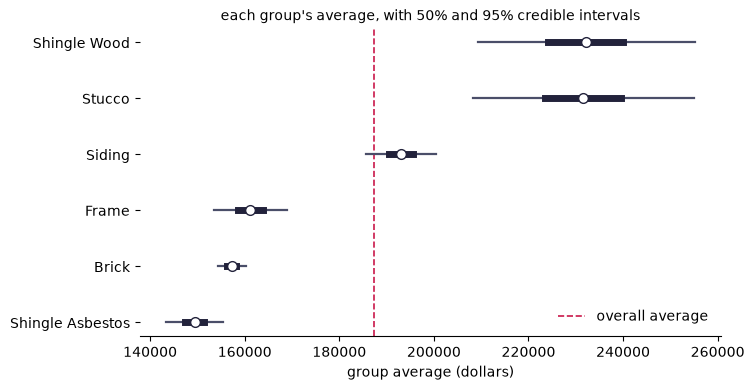
print(res_groups.pairwise(only=[("Stucco", "Brick"), ("Frame", "Brick")]))
PAIRWISE COMPARISONS (partially pooled)

comparison                    difference  95% interval           P(1st>2nd)
----------------------------------------------------------------------------
Stucco − Brick                74275.96    50774.92 to 97925.59        1.000
Frame − Brick                 3940.42     -4289.47 to 12177.94        0.826

comparison                      BF10 (JZS)   verdict
----------------------------------------------------------------------------
Stucco − Brick                 93470477.31   favours a difference
Frame − Brick                         0.06   favours no difference

Note: Every row is an estimate, not a test, so no multiple-comparisons
      correction is applied or needed. Describing several groups does not
      make the description of any one of them less accurate. If you are
      worried that a small group looks extreme by chance, the fix is
      pool=True, not a correction.
res_groups.plot(kind="forest");
import pandas as pd

table = pd.crosstab(parcels.construction, parcels.condition)
print(bp.contingency(table).summary())
==========================================================================
 strength of association (Cramér's V) between rows and columns
==========================================================================

 BAYESIAN — what the data say about the quantity itself

   best estimate (median)    0.078
   95% credible interval     0.064 to 0.092  (HDI)
   P(above 0.100)            0.002

   Read: The best estimate of the association strength is 0.078, and the
         data are consistent with anything from 0.064 to 0.092 (95%
         credible interval).

 FREQUENTIST — Pearson chi-square test of independence

   chi-square (15 df)        123.9
   p-value                   3.337e-19  (significant at 0.05)

   Read: If rows and columns were unrelated, data at least this extreme
         would turn up less than once in a million studies.

   --------------------------------------------------------------------

   How they line up
     They are not aimed at the same target. The test asks whether rows
     and columns were unrelated, and rules it out at p = 3.34e-19. The
     posterior does not measure against that hypothesis at all: it
     measures against 0.100, a conventional bar for a small effect. So
     the test tells you there is something here, and the interval —
     0.064 to 0.092 — tells you how much. With data this plentiful the
     first question is nearly always settled, which is why the second
     one is the one worth reporting.

--------------------------------------------------------------------------
 assumption   prior: uninformed — Dirichlet(1)
 precision    100,000 independent draws; Monte Carlo error on the mean
              is ±2.3e-05. These are exact samples, not a Markov chain.
 note         Cramér's V cannot be negative, so P(above 0.1) is measured
              against a conventional 'small association' bar rather than a
              null. Set threshold= to a value that matters for your
              decision instead.
 next         .probability('>', x)  .decide(rope=(lo, hi))  .sensitivity()
==========================================================================
tracts = bp.datasets.load_tracts().dropna(subset=["median_income", "median_rent"])
corr = bp.correlation(
    tracts.median_income, tracts.median_rent,
    labels=["median income", "median rent"], aggregated=True,
)
corr.sentence()
'The best estimate of the correlation is 0.781, and the data are consistent with anything from 0.765 to 0.796 (95% credible interval).'
Rates
A count over an exposure is a rate, not a proportion. Deaths per thousand collisions, by county:
collisions = bp.datasets.load_collisions()
by_county = collisions.groupby("county").agg(
    killed=("killed", "sum"), crashes=("killed", "size")
)
deaths = bp.compare_rates(
    events=by_county.killed.to_numpy(),
    exposure=by_county.crashes.to_numpy() / 1000,
    labels=list(by_county.index),
    unit="per 1,000 collisions",
)
deaths.sentence()
'San Diego is higher than Los Angeles with 99% probability; the best estimate of the ratio is 1.83 times, and the data are consistent with anything from 1.00 to 2.85 times (95% credible interval).'
The rate ratio’s posterior is exact, so there is nothing to sample. Pass
per-period counts to rate() and it also checks whether they vary more than a
steady rate allows. These do, by a lot, and the result says so:
per_year = collisions[collisions.county == "Los Angeles"].groupby("year").size()
bp.rate(per_year.to_numpy(), reference=2000, unit="per year").notes[0]
'the counts vary between periods about 107.0 times as much as a steady rate would produce (dispersion test p = 2.4e-91). The rate is probably not steady, and this interval understates the uncertainty — report it as a lower bound on how uncertain you are'
One categorical variable
Does each county’s share of collisions match its share of the two counties’ population, roughly three to one?
shares = bp.categories(
    collisions.county, expected={"Los Angeles": 0.75, "San Diego": 0.25}
)
print(shares.shares())
EACH CATEGORY AGAINST ITS EXPECTED SHARE

category            count  expected  estimate      95% interval  P(above)
--------------------------------------------------------------------------
Los Angeles         9,886     75.0%     82.4%    81.7% to 83.1%     1.000  *
San Diego           2,114     25.0%     17.6%    16.9% to 18.3%     0.000  *

Note: * the 95% interval excludes the expected share. P(above) is the
      probability the category's true share is higher than expected. Each
      row is an estimate, not a test, so no correction for looking at
      several categories is needed.
A line with one predictor
line = bp.regression(
    parcels.sqft, parcels.assessed_value,
    labels=["floor area", "assessed value"], unit="dollars per sq ft",
)
line.sentence()
'The best estimate of the slope is 117.35 dollars per sq ft, and the data are consistent with anything from 113.75 to 120.95 dollars per sq ft (95% credible interval).'
Paired data, and skewed data
compare_means(..., paired=True) compares two measurements on the same units
and reports how much the pairing narrowed the interval.
compare_means(..., log=True) answers in ratios of typical values, which suits
prices and incomes:
bp.compare_means(
    rowhouses, detached, labels=["rowhouse", "detached"], log=True
).sentence()
'detached is higher than rowhouse with 70% probability; the best estimate of the ratio is 1.01 times, and the data are consistent with anything from 0.97 to 1.05 times (95% credible interval).'
Forecasting the next one
.predict() forecasts the next observation, carrying the uncertainty in the
estimate through. It prints the plug-in forecast next to it, which treats the
estimate as exact and is always too narrow:
print(bp.proportion(3, 12).predict(n=100))
==========================================================================
 forecast: number of successes in the next 100 cases
==========================================================================

   median                    27
   95% forecast interval     8 to 56
   plug-in interval          17 to 34  (estimate treated as exact)

   Read: The number of successes in the next 100 cases is forecast at
         about 27 (the median), and there is a 95% probability it lands in
         the range 8 to 56.

   Why: The plug-in interval is narrower because it treats the estimate as
        if it were known exactly, so it carries only the ordinary
        variation in the outcome. The forecast above also carries the
        uncertainty in the estimate itself. The gap between them shrinks
        as the data grow; with little data it is the larger part of the
        story.
==========================================================================
Reproducibility in a classroom
The seed is fixed by default, so every student sees identical digits:
bp.get_seed(), bp.get_draws()
(12345, 100000)
Having hidden that noise, the package surfaces it — every sampled quantity
prints its Monte Carlo standard error. Use bp.set_seed(None) to show a class
that the wobble is real.