How to run Bayesian LM specification tests¶

You have a spatial dataset and need to decide which model to fit: is the dependence in the outcome (a lag), in the errors, in the neighbours’ covariates, or some combination? The Lagrange-Multiplier tests answer that before you commit to a specification.

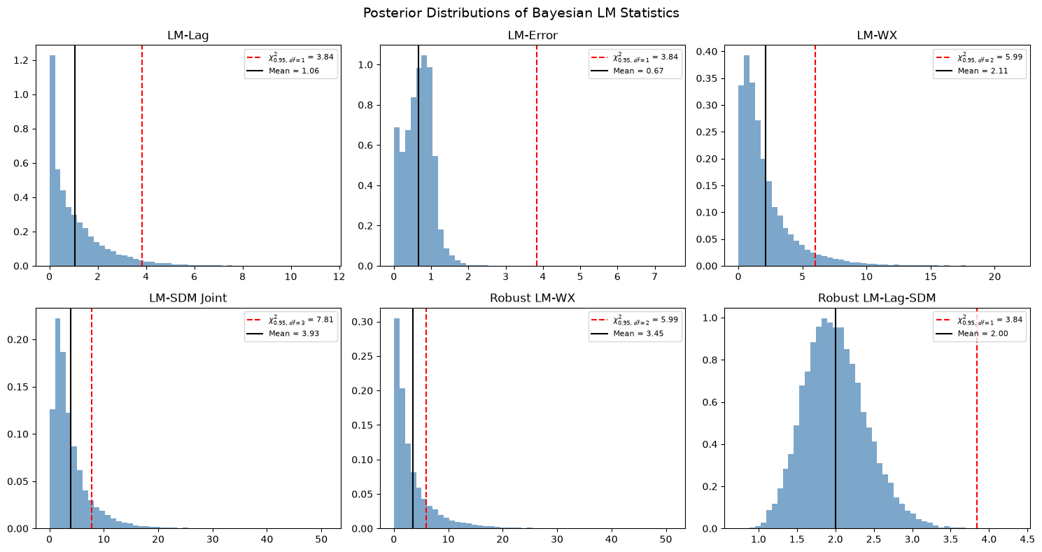
neighbayes evaluates each LM statistic at every posterior draw, so you get a posterior distribution of the statistic rather than a single point. The full inventory of tests, their null hypotheses and degrees of freedom, and the Neyman-orthogonal construction behind the robust variants are in Supported Models.

import warnings

import libpysal
import matplotlib.pyplot as plt
import numpy as np
import pandas as pd

from neighbayes.diagnostics.lmtests import (
    bayesian_lm_error_sdm_test,
    bayesian_lm_error_test,
    bayesian_lm_lag_sdem_test,
    bayesian_lm_lag_test,
    bayesian_lm_sdm_joint_test,
    bayesian_lm_slx_error_joint_test,
    bayesian_lm_wx_sem_test,
    bayesian_lm_wx_test,
    bayesian_robust_lm_error_sdem_test,
    bayesian_robust_lm_error_test,
    bayesian_robust_lm_lag_sdm_test,
    bayesian_robust_lm_lag_test,
    bayesian_robust_lm_wx_test,
)
from neighbayes.models import OLS, SAR, SDEM, SDM, SEM, SLX

warnings.filterwarnings("ignore", category=FutureWarning)
warnings.filterwarnings("ignore", category=UserWarning)

/home/runner/micromamba/envs/test/lib/python3.14/site-packages/tqdm/auto.py:21: TqdmWarning: IProgress not found. Please update jupyter and ipywidgets. See https://ipywidgets.readthedocs.io/en/stable/user_install.html
  from .autonotebook import tqdm as notebook_tqdm

Set up data and weights¶

We create a simple spatial DGP with known parameters to validate the tests. Under the null hypothesis (no spatial effects), the Bayesian LM statistics should be small with high p-values.

import geopandas as gpd
from libpysal.graph import Graph
from libpysal.weights import Rook

# Generate data under H0: no spatial effects
np.random.seed(42)

# Load Columbus dataset for spatial weights
columbus_path = libpysal.examples.get_path("columbus.shp")
gdf = gpd.read_file(columbus_path)

# Create a Graph (modern libpysal API) for neighbayes models
# Row-standardize the graph so spatial models work correctly
g = Graph.build_contiguity(gdf, rook=True).transform("r")
n = g.n

# Legacy W for spreg comparison
w_spreg = Rook.from_shapefile(columbus_path)
w_spreg.transform = "r"

# Get sparse and dense W matrices
W_sparse = g.sparse.tocsr().astype(np.float64)
W_dense = np.array(W_sparse.todense())

# Design matrix
k = 3
X = np.column_stack([np.ones(n), np.random.normal(size=(n, k - 1))])
beta_true = np.array([1.0, 2.0, -1.5])
y = X @ beta_true + np.random.normal(scale=1.0, size=n)

print(f"W shape: {W_sparse.shape}, nnz: {W_sparse.nnz}")

W shape: (49, 49), nnz: 200

Fit the null models the tests need¶

The Bayesian LM tests require posterior draws from the null model (the model under H₀). Different tests use different null models:

LM-WX test: SAR model (includes ρ but not γ)
LM-SDM joint test: OLS model (no spatial params)
LM-SLX-Error joint test: OLS model (no spatial params)
Robust LM-Lag-SDM: SLX model (includes γ but not ρ)
Robust LM-WX: SAR model (includes ρ but not γ)
Robust LM-Error-SDEM: SLX model (includes γ but not λ)

# Fit OLS model (null for joint tests)
ols_model = OLS(y=y, X=X, W=g)
ols_model.fit(draws=5000, tune=5000, chains=4, random_seed=42)

# Fit SAR model (null for LM-WX and robust LM-WX)
sar_model = SAR(y=y, X=X, W=g)
sar_model.fit(draws=5000, tune=5000, chains=4, random_seed=42)

# Fit SLX model (null for robust LM-Lag-SDM and robust LM-Error-SDEM)
slx_model = SLX(y=y, X=X, W=g)
slx_model.fit(draws=5000, tune=5000, chains=4, random_seed=42)

Initializing NUTS using jitter+adapt_diag...
Multiprocess sampling (4 chains in 2 jobs)
NUTS: [beta, sigma2]
Sampling 4 chains for 5_000 tune and 5_000 draw iterations (20_000 + 20_000 draws total) took 17 seconds.
/home/runner/micromamba/envs/test/lib/python3.14/site-packages/neighbayes/_logdet/_jax.py:188: ComplexWarning: Casting complex values to real discards the imaginary part
  W_arr = np.asarray(W, dtype=np.float64)
Initializing NUTS using jitter+adapt_diag...
Multiprocess sampling (4 chains in 2 jobs)
NUTS: [beta, sigma2]
Sampling 4 chains for 5_000 tune and 5_000 draw iterations (20_000 + 20_000 draws total) took 18 seconds.

Gibbs sampling (sar): 4 chains for 5,000 tune and 5,000 draw iterations (4 x 10,000 = 40,000 draws total)

Sampling took 4s (9,653 draws/s)

arviz.InferenceData

Test for a lag, an error, or lagged covariates¶

These tests assume the nuisance parameters are correctly specified (zero). They are the Bayesian analogues of the classical LM tests from Koley & Bera (2024).

# Fit the SEM null required by LM-WX-SEM (Bayesian analogue of Koley–Bera 2024).
sem_model = SEM(y=y, X=X, W=g)
sem_model.fit(draws=2500, tune=2500, chains=2, random_seed=42)

# Non-robust Bayesian LM tests evaluated at the appropriate null model.
non_robust_results = pd.DataFrame(
    [
        bayesian_lm_lag_test(ols_model).to_series(),
        bayesian_lm_error_test(ols_model).to_series(),
        bayesian_lm_wx_test(sar_model).to_series(),
        bayesian_lm_wx_sem_test(sem_model).to_series(),
        bayesian_lm_sdm_joint_test(ols_model).to_series(),
        bayesian_lm_slx_error_joint_test(ols_model).to_series(),
    ],
    index=[
        "LM-Lag",
        "LM-Error",
        "LM-WX",
        "LM-WX-SEM",
        "LM-SDM Joint",
        "LM-SLX-Error Joint",
    ],
)

non_robust_results

/home/runner/micromamba/envs/test/lib/python3.14/site-packages/neighbayes/_logdet/_jax.py:188: ComplexWarning: Casting complex values to real discards the imaginary part
  W_arr = np.asarray(W, dtype=np.float64)

Gibbs sampling (sem): 2 chains for 2,500 tune and 2,500 draw iterations (2 x 5,000 = 10,000 draws total)

Sampling took 4s (2,792 draws/s)

	lm_samples	mean	median	credible_interval	bayes_pvalue	test_type	df	n_draws	k_wx
LM-Lag	[0.2142964999714562, 1.0784033337488124, 1.280...	1.063234	0.656830	(0.00204675682175708, 4.2687677969034805)	0.302479	bayesian_lm_lag	1	20000	NaN
LM-Error	[0.7079187163674764, 0.7756572487282847, 0.744...	0.669052	0.683859	(0.014393878917328799, 1.3853911845443372)	0.413382	bayesian_lm_error	1	20000	NaN
LM-WX	[1.4814399069845414, 3.360987014281438, 0.8809...	2.112357	1.413838	(0.09593622926595723, 8.194730280544038)	0.347782	bayesian_lm_wx	2	20000	2.0
LM-WX-SEM	[3.2315485732635807, 1.0743489513363125, 0.196...	1.351305	0.898337	(0.05536302605253931, 5.110249054287485)	0.508824	bayesian_lm_wx_sem	2	5000	2.0
LM-SDM Joint	[0.7240693263411846, 2.7662057621909844, 2.499...	3.926935	2.786218	(0.42552310256782655, 14.128384100207635)	0.269463	bayesian_lm_sdm_joint	3	20000	2.0
LM-SLX-Error Joint	[1.3998088300832858, 3.5034345838334366, 1.597...	2.113251	1.633809	(0.7011929236378855, 6.1492522670831296)	0.549237	bayesian_lm_slx_error_joint	3	20000	2.0

Use the robust variants when both channels may be present¶

These tests use the Neyman orthogonal score adjustment from Dogan et al. (2021, Proposition 3) to ensure robustness against local misspecification in the nuisance parameter. This is the key innovation over the classical Bera-Yoon (1993) approach.

The adjustment removes the correlation between the test parameter score and the nuisance parameter score:

\[g_\psi^* = g_\psi - J_{\psi\phi \cdot \sigma} \, J_{\phi\phi \cdot \sigma}^{-1} \, g_\phi\]

where \(J_{\cdot \cdot \cdot \sigma}\) denotes information matrix blocks partitioned on \(\sigma^2\).

# Robust Bayesian LM tests (Neyman orthogonal score)
robust_results = pd.DataFrame(
    [
        bayesian_robust_lm_lag_test(ols_model).to_series(),
        bayesian_robust_lm_error_test(ols_model).to_series(),
        bayesian_robust_lm_lag_sdm_test(slx_model).to_series(),
        bayesian_robust_lm_wx_test(sar_model).to_series(),
        bayesian_robust_lm_error_sdem_test(slx_model).to_series(),
    ],
    index=[
        "Robust LM-Lag",
        "Robust LM-Error",
        "Robust LM-Lag-SDM",
        "Robust LM-WX",
        "Robust LM-Error-SDEM",
    ],
)

robust_results

	lm_samples	mean	median	credible_interval	bayes_pvalue	test_type	df	n_draws	k_wx	tr_MzWMzW_pair
Robust LM-Lag	[0.04470652999465163, 0.06039321001634612, 0.0...	0.052556	0.049121	(0.021080445691699274, 0.10259303831611782)	0.818673	bayesian_robust_lm_lag	1	20000	NaN	NaN
Robust LM-Error	[0.2592088833186119, 0.35016040229998335, 0.23...	0.304723	0.284806	(0.12222462329905084, 0.5948354055071119)	0.580937	bayesian_robust_lm_error	1	20000	NaN	NaN
Robust LM-Lag-SDM	[1.497849382284626, 1.7175227063115825, 1.8123...	2.003181	1.974842	(1.2853662789897897, 2.877608504387878)	0.156969	bayesian_robust_lm_lag_sdm	1	20000	2.0	19.966602
Robust LM-WX	[2.548722904936673, 2.5345872759229016, 0.1998...	3.448256	1.918213	(0.08724517028584271, 15.464011910652697)	0.178328	bayesian_robust_lm_wx	2	20000	2.0	NaN
Robust LM-Error-SDEM	[1.4121519102807134, 1.6051095505017356, 1.687...	1.844711	1.826631	(1.222114877277616, 2.565960814166178)	0.174400	bayesian_robust_lm_error_sdem	1	20000	2.0	19.966602

Read the whole posterior, not just the point statistic¶

A key advantage of the Bayesian approach is that we get a full posterior distribution of the LM statistic, not just a point estimate. This allows us to compute credible intervals and posterior probabilities.

from scipy import stats as sp_stats

# Show six representative posterior LM distributions (a mix of non-robust and
# robust variants).  Each panel overlays the chi-squared 95% reference and the
# posterior mean.
panels = [
    ("LM-Lag", bayesian_lm_lag_test(ols_model)),
    ("LM-Error", bayesian_lm_error_test(ols_model)),
    ("LM-WX", bayesian_lm_wx_test(sar_model)),
    ("LM-SDM Joint", bayesian_lm_sdm_joint_test(ols_model)),
    ("Robust LM-WX", bayesian_robust_lm_wx_test(sar_model)),
    ("Robust LM-Lag-SDM", bayesian_robust_lm_lag_sdm_test(slx_model)),
]

fig, axes = plt.subplots(2, 3, figsize=(15, 8))
for ax, (name, res) in zip(axes.flat, panels):
    ax.hist(res.lm_samples, bins=50, density=True, alpha=0.7, color="steelblue")
    chi2_ref = sp_stats.chi2.ppf(0.95, res.df)
    ax.axvline(
        chi2_ref,
        color="red",
        linestyle="--",
        label=f"$\\chi^2_{{0.95,\\,df={res.df}}}$ = {chi2_ref:.2f}",
    )
    ax.axvline(res.mean, color="black", linestyle="-", label=f"Mean = {res.mean:.2f}")
    ax.set_title(name)
    ax.legend(fontsize=8)

plt.suptitle("Posterior Distributions of Bayesian LM Statistics", fontsize=14)
plt.tight_layout()
plt.show()

../_images/36197f1eca6d89d07c0bc89d68e003a1d38fad399d036f2d5e5ae0f16bbe9208.png

Get a recommendation instead of a table¶

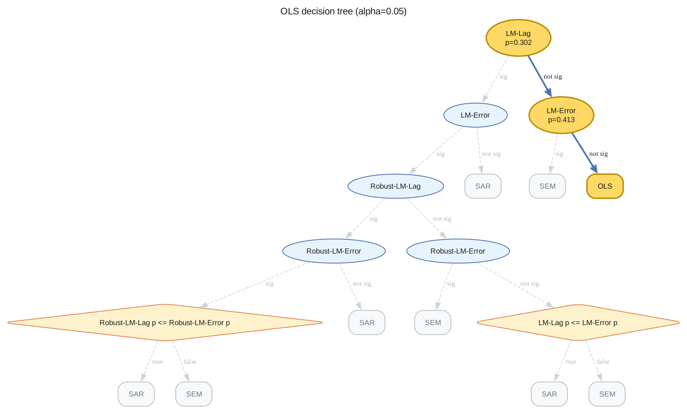
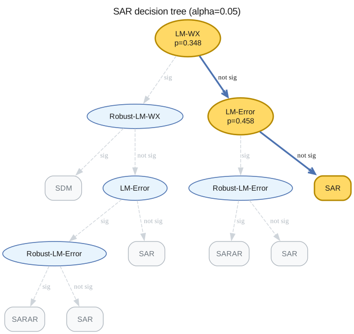
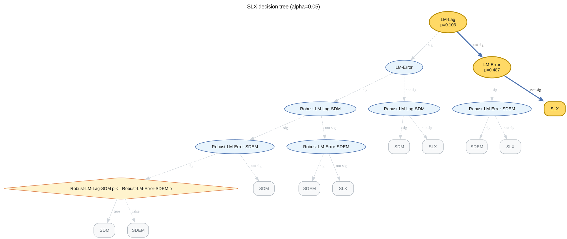
Every fitted spatial model exposes spatial_diagnostics() and spatial_diagnostics_decision(). The registry on each class wires the correct tests for its specification:

OLS → LM-Lag, LM-Error, LM-SDM-Joint, LM-SLX-Error-Joint, Robust-LM-Lag, Robust-LM-Error
SAR → LM-Error, LM-WX, Robust-LM-WX
SEM → LM-Lag, LM-WX
SLX → LM-Lag, LM-Error, Robust-LM-Lag-SDM, Robust-LM-Error-SDEM
SDM → LM-Error-SDM (uses correct \(e = y - \rho Wy - X\beta - WX\gamma\) residuals)
SDEM → LM-Lag-SDEM (uses \((I-\lambda W)\)-filtered residuals)

# Method-based API: one call returns all wired tests as a DataFrame
ols_model.spatial_diagnostics()

	statistic	median	df	p_value	ci_lower	ci_upper
test
LM-Lag	1.063234	0.656830	1	0.302479	0.002047	4.268768
LM-Error	0.669052	0.683859	1	0.413382	0.014394	1.385391
LM-SDM-Joint	3.926935	2.786218	3	0.269463	0.425523	14.128384
LM-SLX-Error-Joint	2.113251	1.633809	3	0.549237	0.701193	6.149252
Robust-LM-Lag	0.052556	0.049121	1	0.818673	0.021080	0.102593
Robust-LM-Error	0.304723	0.284806	1	0.580937	0.122225	0.594835

# The decision routine walks the appropriate tests and returns a recommendation
print("OLS recommends:")
ols_model.spatial_diagnostics_decision()

OLS recommends:

../_images/41e10602260842b0bb62a105ccdbca0fd4ce42ae530106f419823233e17ad4af.svg

print("SAR recommends:")
sar_model.spatial_diagnostics_decision()

SAR recommends:

../_images/4668d574474b2fdc181c242d27ca3d95076d9eb4ab01945aed0ba92ef82e4c7a.svg

print("SLX recommends:")
slx_model.spatial_diagnostics_decision()

SLX recommends:

../_images/03ff809b58bc2a8f565b609da2610e569b8c7b213176a0b3a4580e78b4a9c0dd.svg

# SDM/SDEM-aware tests require fitted SDM / SDEM models so the residuals
# include the correct spatial filters.
sdm_model = SDM(y=y, X=X, W=g)
sdm_model.fit(draws=2000, tune=2000, chains=2, random_seed=42)

sdem_model = SDEM(y=y, X=X, W=g)
sdem_model.fit(draws=2000, tune=2000, chains=2, random_seed=42)

pd.DataFrame(
    [
        bayesian_lm_error_sdm_test(sdm_model).to_series(),
        bayesian_lm_lag_sdem_test(sdem_model).to_series(),
    ],
    index=["LM-Error-SDM", "LM-Lag-SDEM"],
)

/home/runner/micromamba/envs/test/lib/python3.14/site-packages/neighbayes/_logdet/_jax.py:188: ComplexWarning: Casting complex values to real discards the imaginary part
  W_arr = np.asarray(W, dtype=np.float64)

Gibbs sampling (sdm): 2 chains for 2,000 tune and 2,000 draw iterations (2 x 4,000 = 8,000 draws total)

Sampling took 3s (2,534 draws/s)

Gibbs sampling (sdem): 2 chains for 2,000 tune and 2,000 draw iterations (2 x 4,000 = 8,000 draws total)

Sampling took 3s (2,296 draws/s)

	lm_samples	mean	median	credible_interval	bayes_pvalue	test_type	df	n_draws
LM-Error-SDM	[0.32821317533390937, 0.1084400084000235, 0.35...	1.163491	0.330490	(0.0005711733395424328, 7.945960590111098)	0.280743	bayesian_lm_error_sdm	1	4000
LM-Lag-SDEM	[5.220403887297558, 3.5843989225132207, 0.0223...	1.923766	0.835193	(0.001694640195268472, 9.986359293919964)	0.165442	bayesian_lm_lag_sdem	1	4000

Run the same tests on panel data¶

The same Bayesian LM machinery extends to balanced spatial panels. Tests of the form bayesian_panel_lm_* and bayesian_panel_robust_lm_* are wired into every panel model (OLSPanelFE, SARPanelFE, SLXPanelFE, …) and surfaced through the same spatial_diagnostics() / spatial_diagnostics_decision() methods.

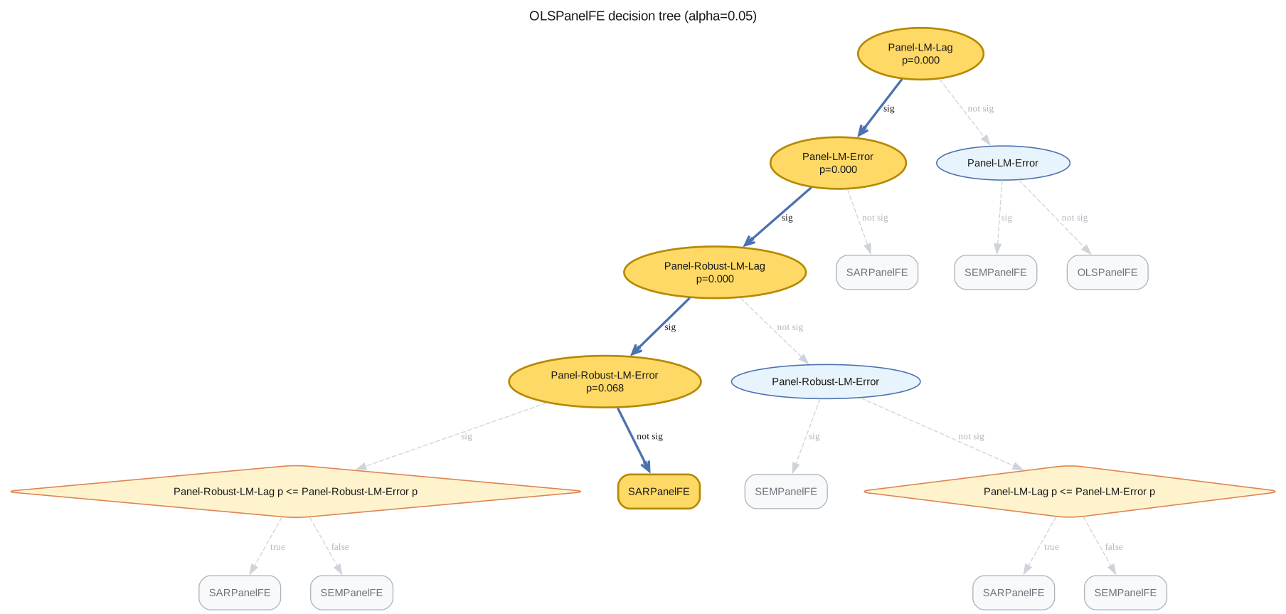
Below we simulate a small balanced panel (\(N = 81\), \(T = 4\)) from the panel fixed-effects OLS DGP and run the full diagnostic table.

from neighbayes.dgp.panel_fe import simulate_panel_sar_fe
from neighbayes.dgp.utils import rook_grid_weights
from neighbayes.models import OLSPanelFE

# 9x9 rook grid (N=81), T=4 — small enough to fit quickly but large enough for
# the LM tests to behave well.
N_panel, T_panel = 81, 4
W_panel_dense, W_panel_graph = rook_grid_weights(int(np.sqrt(N_panel)))

# Simulate from a SAR-FE DGP with moderate spatial dependence so the LM-Lag
# direction is clearly significant.
panel_sim = simulate_panel_sar_fe(
    N=N_panel,
    T=T_panel,
    rho=0.4,
    beta=np.array([1.0, 2.0]),
    W=W_panel_graph,
    seed=11,
)

panel_model = OLSPanelFE(
    y=panel_sim["y"],
    X=panel_sim["X"],
    W=W_panel_graph,
    N=N_panel,
    T=T_panel,
    effects=3,  # two-way fixed effects (unit + time)
)
panel_model.fit(draws=600, tune=600, chains=2, random_seed=11, progressbar=False)

panel_model.spatial_diagnostics()

Initializing NUTS using jitter+adapt_diag...
Multiprocess sampling (2 chains in 2 jobs)
NUTS: [beta, sigma2]
Sampling 2 chains for 600 tune and 600 draw iterations (1_200 + 1_200 draws total) took 5 seconds.
We recommend running at least 4 chains for robust computation of convergence diagnostics

	statistic	median	df	p_value	ci_lower	ci_upper
test
Panel-LM-Lag	84.694264	84.656800	1	0.000000e+00	77.426851	91.951679
Panel-LM-Error	22.321703	21.940709	1	2.305858e-06	11.806254	34.658109
Panel-LM-SDM-Joint	88.138628	88.039371	2	0.000000e+00	82.867041	93.807878
Panel-LM-SLX-Error-Joint	88.422994	88.041710	2	0.000000e+00	78.285630	100.394412
Panel-Robust-LM-Lag	67.184064	66.740233	1	2.220446e-16	47.935579	91.675476
Panel-Robust-LM-Error	3.341650	3.319574	1	6.754686e-02	2.384254	4.559821

print(
    f"Panel decision tree (DGP = SAR-FE) recommends: {panel_model.spatial_diagnostics_decision(alpha=0.05, format='model')}"
)

Panel decision tree (DGP = SAR-FE) recommends: SARPanelFE

panel_model.spatial_diagnostics_decision(
    alpha=0.05,
)

../_images/90a63d09fdf8f38877bd1129d452a12da263269bc94146faa6d3b83430e91b87.svg

Run them on origin–destination flows¶

Origin–destination flow models in neighbayes.models.flow use Kronecker weight matrices \(W_d, W_o, W_w\) for destination, origin, and network spillovers respectively. The Bayesian LM family for flows tests each direction separately (bayesian_lm_flow_dest_test, bayesian_lm_flow_orig_test, bayesian_lm_flow_network_test, bayesian_lm_flow_intra_test) plus a joint test (bayesian_lm_flow_joint_test). Robust variants are available for the destination, origin, and network directions.

The registry on OLSFlow wires the full set; SARFlow (which already includes all three lag terms) wires the robust variants for marginal-extension testing.

from neighbayes.dgp.flows import generate_flow_data
from neighbayes.models import OLSFlow, SARFlow

# Simulate a small SAR flow DGP on n=8 spatial units (N = 64 OD cells).
flow_data = generate_flow_data(
    n=8,
    rho_d=0.35,
    rho_o=0.25,
    rho_w=0.10,
    beta_d=[1.0, -0.5],
    beta_o=[0.5, 0.3],
    sigma=1.0,
    seed=42,
)

y_flow = np.log(flow_data["y_vec"])  # latent SAR scale (DGP default is lognormal)
X_flow = flow_data["X"]
G_flow = flow_data["G"]

ols_flow = OLSFlow(y_flow, X_flow, G_flow, col_names=flow_data["col_names"])
ols_flow.fit(draws=600, tune=600, chains=2, random_seed=42, progressbar=False)

ols_flow.spatial_diagnostics()

Initializing NUTS using jitter+adapt_diag...
Multiprocess sampling (2 chains in 2 jobs)
NUTS: [beta, sigma]
Sampling 2 chains for 600 tune and 600 draw iterations (1_200 + 1_200 draws total) took 6 seconds.
We recommend running at least 4 chains for robust computation of convergence diagnostics

	statistic	median	df	p_value	ci_lower	ci_upper
test
LM-Flow-Dest	0.449894	0.212377	1	0.502386	0.000395	2.271064
LM-Flow-Orig	0.628676	0.337023	1	0.427842	0.000724	2.949834
LM-Flow-Network	0.430998	0.184981	1	0.511499	0.000299	2.296940
LM-Flow-Joint	1.535489	1.165474	3	0.674104	0.117953	5.115903
LM-Flow-Intra	1.171645	0.916407	3	0.759813	0.071717	3.916607

flow_data.keys()

dict_keys(['y_vec', 'y_mat', 'eta_vec', 'eta_mat', 'distribution', 'X', 'X_regional', 'X_regional_d', 'X_regional_o', 'col_names', 'design', 'W', 'G', 'gdf', 'dist', 'rho_d', 'rho_o', 'rho_w', 'sigma', 'beta_d', 'beta_o', 'gamma_dist'])

# Fit the SAR flow alternative; its diagnostic registry consists of the robust
# (Neyman-orthogonal) marginal-extension tests.
sar_flow = SARFlow(y_flow, X_flow, G_flow, col_names=flow_data["col_names"])
sar_flow.fit(draws=600, tune=600, chains=2, random_seed=42, progressbar=False)

sar_flow.spatial_diagnostics()

	statistic	median	df	p_value	ci_lower	ci_upper
test
Robust-LM-Flow-Dest	0.412042	0.192364	1	0.520935	0.000334	2.034098
Robust-LM-Flow-Orig	0.466157	0.226649	1	0.494761	0.000478	2.252824
Robust-LM-Flow-Network	0.551544	0.269556	1	0.457688	0.000538	2.493822
LM-Flow-Intra	1.407651	1.131638	3	0.703742	0.100356	4.479055