Getting Started with neighbayes
This notebook walks through a complete spatial econometric workflow:
Simulate spatial data from a known DGP
Fit a baseline OLS model
Run Bayesian LM diagnostics to test for spatial dependence
Use the decision tree to select a better model
Fit the recommended SAR model
Compute direct, indirect, and total spatial effects
Peek at the underlying PyMC model for customization
import libpysal

from neighbayes.dgp import simulate_sar

gdf = simulate_sar(n=20, beta=[1, 0.4, 2.5], rho=0.6, create_gdf=True)
gdf
| y | X_0 | X_1 | X_2 | geometry | |
|---|---|---|---|---|---|
| 0 | -0.813218 | 1.0 | -0.775638 | -0.774242 | POLYGON ((1 0, 1 1, 0 1, 0 0, 1 0)) |
| 1 | -2.942186 | 1.0 | -1.465023 | -1.171733 | POLYGON ((2 0, 2 1, 1 1, 1 0, 2 0)) |
| 2 | 0.003527 | 1.0 | -1.596144 | -0.454324 | POLYGON ((3 0, 3 1, 2 1, 2 0, 3 0)) |
| 3 | 1.945309 | 1.0 | 0.071310 | 0.556691 | POLYGON ((4 0, 4 1, 3 1, 3 0, 4 0)) |
| 4 | 5.211010 | 1.0 | 0.114352 | 0.305765 | POLYGON ((5 0, 5 1, 4 1, 4 0, 5 0)) |
| ... | ... | ... | ... | ... | ... |
| 395 | 0.346182 | 1.0 | -1.133226 | 0.664088 | POLYGON ((16 19, 16 20, 15 20, 15 19, 16 19)) |
| 396 | -2.586067 | 1.0 | 2.037456 | -1.572567 | POLYGON ((17 19, 17 20, 16 20, 16 19, 17 19)) |
| 397 | 1.051976 | 1.0 | 0.177340 | -0.574260 | POLYGON ((18 19, 18 20, 17 20, 17 19, 18 19)) |
| 398 | 10.023798 | 1.0 | 0.109630 | 1.845905 | POLYGON ((19 19, 19 20, 18 20, 18 19, 19 19)) |
| 399 | 6.520899 | 1.0 | 0.053479 | 0.409256 | POLYGON ((20 19, 20 20, 19 20, 19 19, 20 19)) |
400 rows × 5 columns
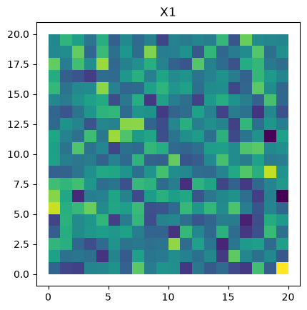
gdf.plot("X_1").set_title("X1")
Text(0.5, 1.0, 'X1')
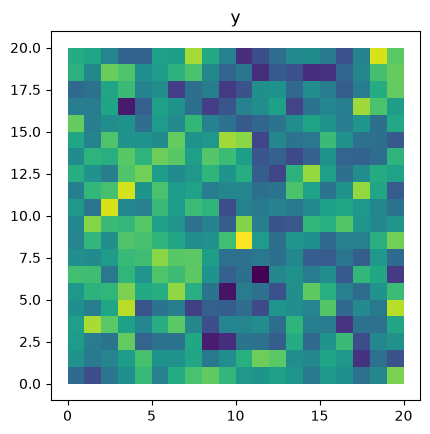
gdf.plot("y").set_title("y")
Text(0.5, 1.0, 'y')
1. Create a Spatial Weights Matrix
Spatial econometric models require a spatial weights matrix \(W\) that encodes the spatial relationships between observations. Here we use Rook contiguity (regions that share a boundary or vertex are neighbors).
G = libpysal.graph.Graph.build_contiguity(gdf, rook=False).transform("r")
2. Fit a Baseline OLS Model
We start with a non-spatial OLS regression to establish a baseline.
# remove the intercept since we have one (-1)
form = "y ~ -1 + X_0 + X_1 + X_2"
from neighbayes.models import OLS

ols = OLS(formula=form, W=G, data=gdf)
ols.fit(draws=1000, tune=500, chains=2, random_seed=42)
ols.summary()
Initializing NUTS using jitter+adapt_diag...
Multiprocess sampling (2 chains in 2 jobs)
NUTS: [beta, sigma2]
Sampling 2 chains for 500 tune and 1_000 draw iterations (1_000 + 2_000 draws total) took 5 seconds.
We recommend running at least 4 chains for robust computation of convergence diagnostics
/home/runner/micromamba/envs/test/lib/python3.14/site-packages/rich/live.py:260: UserWarning: install "ipywidgets"
for Jupyter support
  warnings.warn('install "ipywidgets" for Jupyter support')
| mean | sd | hdi_3% | hdi_97% | mcse_mean | mcse_sd | ess_bulk | ess_tail | r_hat | |
|---|---|---|---|---|---|---|---|---|---|
| X_0 | 2.241 | 0.081 | 2.094 | 2.391 | 0.002 | 0.002 | 1981.0 | 1418.0 | 1.0 |
| X_1 | 0.509 | 0.080 | 0.357 | 0.649 | 0.002 | 0.002 | 1965.0 | 1504.0 | 1.0 |
| X_2 | 2.682 | 0.078 | 2.541 | 2.832 | 0.002 | 0.002 | 2399.0 | 1578.0 | 1.0 |
| sigma2 | 2.538 | 0.184 | 2.184 | 2.862 | 0.004 | 0.005 | 1743.0 | 1471.0 | 1.0 |
| sigma | 1.592 | 0.057 | 1.487 | 1.700 | 0.001 | 0.001 | 1743.0 | 1471.0 | 1.0 |
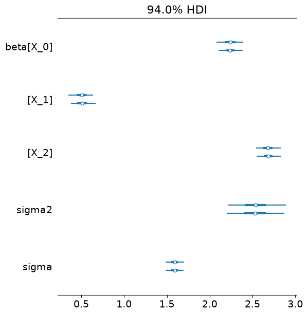
Notice all the estimated beta parameters are biased upward.
Use arviz to inspect fit
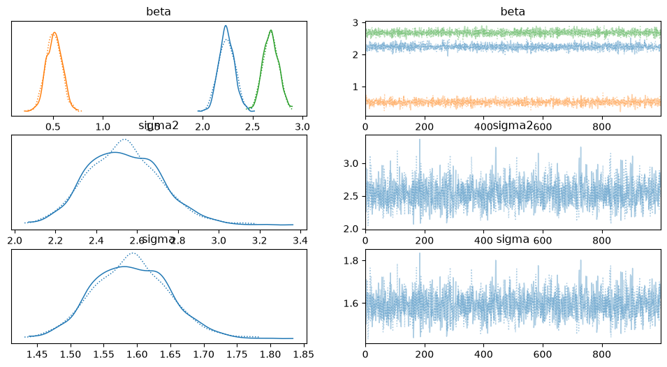
the fit method attaches an inference_data object to each model that can be used directly with arviz functions
import arviz as az

az.plot_forest(ols.inference_data)
array([<Axes: title={'center': '94.0% HDI'}>], dtype=object)
az.plot_trace(ols.inference_data)
array([[<Axes: title={'center': 'beta'}>,
        <Axes: title={'center': 'beta'}>],
       [<Axes: title={'center': 'sigma2'}>,
        <Axes: title={'center': 'sigma2'}>],
       [<Axes: title={'center': 'sigma'}>,
        <Axes: title={'center': 'sigma'}>]], dtype=object)
3. Run Bayesian LM Diagnostics
The spatial_diagnostics() method runs a battery of Bayesian LM tests (Doğan, Taşpınar & Bera 2021) that check whether spatial dependence is present in the residuals.
LM-Lag: Tests \(H_0: \rho = 0\) (no spatial lag on \(y\))
LM-Error: Tests \(H_0: \lambda = 0\) (no spatial error correlation)
LM-SDM-Joint: Joint test for \(\rho = 0\) and \(\gamma = 0\)
Robust-LM-Lag / Robust-LM-Error: Neyman-orthogonal robust versions
diag = ols.spatial_diagnostics()
diag
/home/runner/micromamba/envs/test/lib/python3.14/site-packages/tqdm/auto.py:21: TqdmWarning: IProgress not found. Please update jupyter and ipywidgets. See https://ipywidgets.readthedocs.io/en/stable/user_install.html
  from .autonotebook import tqdm as notebook_tqdm
| statistic | median | df | p_value | ci_lower | ci_upper | |
|---|---|---|---|---|---|---|
| test | ||||||
| LM-Lag | 341.597863 | 340.015392 | 1 | 0.00000 | 236.356784 | 454.128981 |
| LM-Error | 223.464626 | 222.660718 | 1 | 0.00000 | 177.274172 | 275.049116 |
| LM-SDM-Joint | 362.320818 | 355.920270 | 3 | 0.00000 | 237.012246 | 520.423493 |
| LM-SLX-Error-Joint | 361.003218 | 360.069090 | 3 | 0.00000 | 317.185324 | 410.842873 |
| Robust-LM-Lag | 139.350613 | 137.858420 | 1 | 0.00000 | 103.571825 | 181.737901 |
| Robust-LM-Error | 16.462251 | 16.285970 | 1 | 0.00005 | 12.235507 | 21.469693 |
4. Model Selection Decision Tree
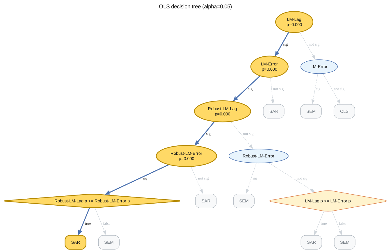
The spatial_diagnostics_decision() method walks a Koley & Bera decision tree using the Bayesian p-values above and recommends the next model to fit.
decision = ols.spatial_diagnostics_decision(alpha=0.05, format="ascii")
print(decision)
LM-Lag *  (p=0.0000, alpha=0.05)
├── <sig> LM-Error *  (p=0.0000, alpha=0.05)
│   ├── <sig> Robust-LM-Lag *  (p=0.0000, alpha=0.05)
│   │   ├── <sig> Robust-LM-Error *  (p=0.0000, alpha=0.05)
│   │   │   ├── <sig> Robust-LM-Lag p <= Robust-LM-Error p *
│   │   │   │   ├── [SAR] * ← SELECTED
│   │   │   │   └── [SEM]
│   │   │   └── [SAR]
│   │   └── <not sig> Robust-LM-Error
│   │       ├── [SEM]
│   │       └── <not sig> LM-Lag p <= LM-Error p
│   │           ├── [SAR]
│   │           └── [SEM]
│   └── [SAR]
└── <not sig> LM-Error
    ├── [SEM]
    └── [OLS]
ols.spatial_diagnostics_decision(alpha=0.05)
5. Fit the Recommended SAR Model
If the diagnostics suggest spatial dependence, we fit a Spatial Autoregressive (SAR) model:
The likelihood includes the Jacobian \(\log|I - \rho W|\) so that posterior inference on \(\rho\) is exact.
from neighbayes.models import SAR

sar = SAR(formula=form, W=G, data=gdf)
sar.fit(draws=2000, tune=100, chains=4, random_seed=42)
sar.summary()
/home/runner/micromamba/envs/test/lib/python3.14/site-packages/neighbayes/_logdet/_jax.py:188: ComplexWarning: Casting complex values to real discards the imaginary part
  W_arr = np.asarray(W, dtype=np.float64)
Gibbs sampling (sar): 4 chains for 100 tune and 2,000 draw iterations (4 x 2,100 = 8,400 draws total)
/home/runner/micromamba/envs/test/lib/python3.14/site-packages/rich/live.py:260: UserWarning: install "ipywidgets"
for Jupyter support
  warnings.warn('install "ipywidgets" for Jupyter support')
Sampling took 4s (1,994 draws/s)
| mean | sd | hdi_3% | hdi_97% | mcse_mean | mcse_sd | ess_bulk | ess_tail | r_hat | |
|---|---|---|---|---|---|---|---|---|---|
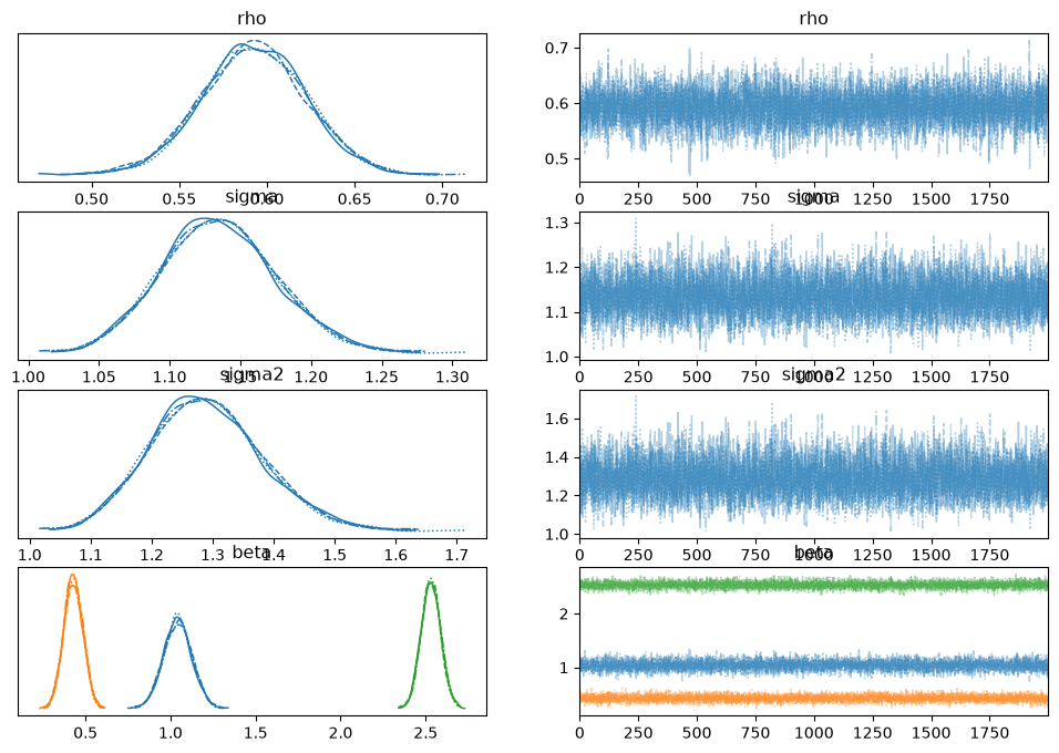
| rho | 0.592 | 0.030 | 0.535 | 0.647 | 0.000 | 0.000 | 8128.0 | 5887.0 | 1.0 |
| sigma | 1.135 | 0.040 | 1.061 | 1.212 | 0.000 | 0.000 | 7590.0 | 7809.0 | 1.0 |
| sigma2 | 1.289 | 0.092 | 1.120 | 1.463 | 0.001 | 0.001 | 7590.0 | 7809.0 | 1.0 |
| X_0 | 1.042 | 0.083 | 0.886 | 1.198 | 0.001 | 0.001 | 7830.0 | 6835.0 | 1.0 |
| X_1 | 0.429 | 0.056 | 0.326 | 0.533 | 0.001 | 0.000 | 7881.0 | 8101.0 | 1.0 |
| X_2 | 2.531 | 0.057 | 2.426 | 2.639 | 0.001 | 0.000 | 7913.0 | 8104.0 | 1.0 |
az.plot_trace(sar.inference_data)
array([[<Axes: title={'center': 'rho'}>, <Axes: title={'center': 'rho'}>],
       [<Axes: title={'center': 'sigma'}>,
        <Axes: title={'center': 'sigma'}>],
       [<Axes: title={'center': 'sigma2'}>,
        <Axes: title={'center': 'sigma2'}>],
       [<Axes: title={'center': 'beta'}>,
        <Axes: title={'center': 'beta'}>]], dtype=object)
6. Compute Spatial Effects
For the SAR model, a change in \(X\) propagates through the spatial multiplier \((I - \rho W)^{-1}\). The effects decompose into:
Direct: Effect of \(X_i\) on \(y_i\) (own-region)
Indirect: Effect of \(X_j\) on \(y_i\) for \(j \neq i\) (spillover)
Total: Direct + Indirect
effects = sar.spatial_effects()
effects
| direct | direct_ci_lower | direct_ci_upper | direct_pvalue | indirect | indirect_ci_lower | indirect_ci_upper | indirect_pvalue | total | total_ci_lower | total_ci_upper | total_pvalue | |
|---|---|---|---|---|---|---|---|---|---|---|---|---|
| variable | ||||||||||||
| X_1 | 0.460241 | 0.343029 | 0.575660 | 0.0 | 0.597216 | 0.403994 | 0.827120 | 0.0 | 1.057457 | 0.761193 | 1.383055 | 0.0 |
| X_2 | 2.718336 | 2.590771 | 2.853071 | 0.0 | 3.526522 | 2.739414 | 4.493698 | 0.0 | 6.244858 | 5.385595 | 7.301870 | 0.0 |