How to choose and configure the Gibbs sampler
fit() already uses Gibbs for the Gaussian spatial models — SAR, SEM, SDM,
SDEM and the Gaussian panel families — because they have a registered Gibbs
sampler and sampler=None prefers it. This guide covers the decisions left to
you: confirming what you got, checking it against NUTS, picking a backend,
loosening the ρ update when it mixes badly, and changing how the
log-determinant is computed.
For the block structure and the full table of backends and log-determinant methods, see Supported Models; for why the conjugate blocks help at all, Architecture.
import time

import arviz as az
import geopandas as gpd
import libpysal
import numpy as np
import pandas as pd

from neighbayes.models import SAR, SDEM, SDM, SEM

gdf = gpd.read_file(libpysal.examples.get_path("columbus.shp"))
y = gdf["CRIME"].values.astype(float)
X = np.column_stack(
    [
        np.ones(len(y)),
        gdf["INC"].values.astype(float),
        gdf["HOVAL"].values.astype(float),
    ]
)
W = libpysal.graph.Graph.build_contiguity(gdf).transform("r")

COMMON = dict(draws=2000, tune=1000, chains=4, random_seed=42)


def fit_timed(model, **kw):
    start = time.perf_counter()
    idata = model.fit(progressbar=False, **kw)
    return idata, time.perf_counter() - start


def efficiency(label, idata, secs, params=("rho", "sigma")):
    ess = az.ess(idata, var_names=list(params))
    rhat = az.rhat(idata, var_names=list(params))
    row = {"seconds": secs}
    for p in params:
        row[f"ess {p}"] = float(ess[p])
        row[f"ess/sec {p}"] = float(ess[p]) / secs
    row["max rhat"] = float(max(float(rhat[p]) for p in params))
    return pd.Series(row, name=label)


print(f"n = {len(y)}, k = {X.shape[1]}")
n = 49, k = 3
Confirm which sampler ran
Nothing in fit() announces its choice, so check the sample_stats group.
A NUTS run carries tree_depth and diverging; a Gibbs run does not.
idata_default, secs_default = fit_timed(SAR(y=y, X=X, W=W), **COMMON)

nuts_only = {"tree_depth", "diverging", "step_size"}
present = nuts_only & set(idata_default.sample_stats.data_vars)
print("sample_stats:", sorted(idata_default.sample_stats.data_vars))
print("ran NUTS" if present else "ran Gibbs")
sample_stats: ['acceptance_rate']
ran Gibbs
/home/runner/micromamba/envs/test/lib/python3.14/site-packages/neighbayes/_logdet/_jax.py:188: ComplexWarning: Casting complex values to real discards the imaginary part
  W_arr = np.asarray(W, dtype=np.float64)
Check the Gibbs result against NUTS
Worth doing once on any new dataset. The two samplers target the same posterior, so a disagreement beyond Monte Carlo error is a defect rather than a tuning difference — and this is the cheapest validation available.
idata_nuts, secs_nuts = fit_timed(
    SAR(y=y, X=X, W=W), sampler="nuts", target_accept=0.9, **COMMON
)

pd.DataFrame(
    {
        "Gibbs": [
            float(idata_default.posterior["rho"].mean()),
            float(idata_default.posterior["sigma"].mean()),
        ],
        "NUTS": [
            float(idata_nuts.posterior["rho"].mean()),
            float(idata_nuts.posterior["sigma"].mean()),
        ],
    },
    index=["rho", "sigma"],
).round(4)
Initializing NUTS using jitter+adapt_diag...
Multiprocess sampling (4 chains in 2 jobs)
NUTS: [rho, beta, sigma2]
Sampling 4 chains for 1_000 tune and 2_000 draw iterations (4_000 + 8_000 draws total) took 15 seconds.
| Gibbs | NUTS | |
|---|---|---|
| rho | 0.4041 | 0.4105 |
| sigma | 10.5043 | 10.5068 |
pd.DataFrame(
    [
        efficiency("Gibbs", idata_default, secs_default),
        efficiency("NUTS", idata_nuts, secs_nuts),
    ]
).round(3)
| seconds | ess rho | ess/sec rho | ess sigma | ess/sec sigma | max rhat | |
|---|---|---|---|---|---|---|
| Gibbs | 4.382 | 7514.982 | 1714.982 | 6721.629 | 1533.932 | 1.001 |
| NUTS | 20.021 | 3989.158 | 199.248 | 4820.380 | 240.765 | 1.000 |
Read the ESS-per-second column, not seconds — a sampler twice as
fast and half as efficient has bought you nothing. Columbus has \(n = 49\); for
timings at realistic sizes see
Performance & Profiling.
Two arguments do not cross the sampler boundary: target_accept raises
TypeError under Gibbs, and idata_kwargs={"log_likelihood": True} is
NUTS-only — Gibbs builds that group unasked.
try:
    SAR(y=y, X=X, W=W).fit(sampler="gibbs", target_accept=0.9, draws=10, tune=10)
except TypeError as err:
    print(f"TypeError: {err}")
TypeError: target_accept is a NUTS-only argument and is not valid for the Gibbs sampler (sampler='gibbs'). Remove it, or use sampler='nuts'.
Pin a backend
gibbs_backend defaults to "auto", which takes JAX when it is installed and
falls back to NumPy. Pin it explicitly when you are benchmarking, or when you
want the NumPy path’s process-level parallelism (n_jobs) instead of the JAX
path’s vectorised chains (chain_method).
pd.DataFrame(
    [
        efficiency(
            backend,
            *fit_timed(
                SAR(y=y, X=X, W=W), sampler="gibbs", gibbs_backend=backend, **COMMON
            ),
        )
        for backend in ("numpy", "jax")
    ]
).round(3)
/home/runner/micromamba/envs/test/lib/python3.14/site-packages/neighbayes/_logdet/_jax.py:188: ComplexWarning: Casting complex values to real discards the imaginary part
  W_arr = np.asarray(W, dtype=np.float64)
| seconds | ess rho | ess/sec rho | ess sigma | ess/sec sigma | max rhat | |
|---|---|---|---|---|---|---|
| numpy | 3.387 | 8206.235 | 2422.59 | 6931.595 | 2046.299 | 1.001 |
| jax | 3.317 | 7514.982 | 2265.75 | 6721.629 | 2026.556 | 1.001 |
JAX pays a one-off compilation cost on the first sweep, so a single small-\(n\) timing is the wrong basis for choosing — at \(n = 49\) that cost is a visible fraction of the total, and at the sizes where you would reach for JAX it is amortized to nothing.
Loosen the ρ update when it mixes poorly
If ess_bulk on ρ or λ is low while β and σ² look fine, the slice sampler’s
interval is the thing to change. slice_width sets its starting width; the
sampler adapts from there during warmup.
idata_tuned, secs_tuned = fit_timed(
    SAR(y=y, X=X, W=W),
    sampler="gibbs",
    gibbs_backend="numpy",
    slice_width=0.25,
    n_jobs=-1,
    thin=2,
    **COMMON,
)
print(f"draws kept per chain with thin=2: {idata_tuned.posterior.sizes['draw']}")
efficiency("slice_width=0.25, thin=2", idata_tuned, secs_tuned).round(3)
draws kept per chain with thin=2: 1000
seconds             3.714
ess rho          3587.911
ess/sec rho       966.077
ess sigma        3983.721
ess/sec sigma    1072.652
max rhat            1.001
Name: slice_width=0.25, thin=2, dtype: float64
Change the log-determinant method
logdet_method goes on the model, not on fit(). Left at None it is
chosen for you by size, by whether \(W\) is symmetric, and by a fill-in estimate;
override it when you know something the selector does not — that your graph
factorizes cheaply, or that it does not.
# The constructor reports the valid names, so this cannot drift out of date.
try:
    SAR(y=y, X=X, W=W, logdet_method="list-them-please")
except ValueError as err:
    print(err)
Unknown logdet method: 'list-them-please'. Valid options: aaa, cheb_cholesky, cheb_stochastic, chebyshev, chol_aaa, cholmod, eigenvalue, grid_spline, lu_cheb, slq, traces.
Verify any approximate method against an exact one before trusting it. On a small problem the exact answer is free, so there is no excuse not to.
pd.DataFrame(
    [
        pd.Series(
            {
                "rho mean": float(idata.posterior["rho"].mean()),
                "rho sd": float(idata.posterior["rho"].std()),
                "seconds": secs,
                "ess rho": float(az.ess(idata, var_names=["rho"])["rho"]),
            },
            name=method,
        )
        for method, (idata, secs) in (
            (
                m,
                fit_timed(
                    SAR(y=y, X=X, W=W, logdet_method=m), sampler="gibbs", **COMMON
                ),
            )
            for m in ("eigenvalue", "chebyshev", "cheb_stochastic")
        )
    ]
).round(4)
/home/runner/micromamba/envs/test/lib/python3.14/site-packages/neighbayes/_logdet/_jax.py:188: ComplexWarning: Casting complex values to real discards the imaginary part
  W_arr = np.asarray(W, dtype=np.float64)
| rho mean | rho sd | seconds | ess rho | |
|---|---|---|---|---|
| eigenvalue | 0.4041 | 0.1252 | 3.3891 | 7514.9820 |
| chebyshev | 0.4033 | 0.1252 | 3.6700 | 7709.4712 |
| cheb_stochastic | 0.4042 | 0.1245 | 3.8732 | 7708.9704 |
eigenvalue is exact at this size, so it is the reference. A method whose
ρ posterior drifts from it is trading accuracy for speed — sometimes the right
trade at scale, never one to make unknowingly.
Apply it to SEM, SDM and SDEM
The same call works for all four Gaussian models; only the name of the spatial
parameter changes (rho for the lag models, lam for the error models).
pd.DataFrame(
    [
        pd.Series(
            {
                "spatial parameter": param,
                "posterior mean": float(idata.posterior[param].mean()),
                "n coefficients": idata.posterior["beta"].sizes["coefficient"],
                "ess": float(az.ess(idata, var_names=[param])[param]),
                "rhat": float(az.rhat(idata, var_names=[param])[param]),
            },
            name=name,
        )
        for name, param, idata in (
            (n, p, fit_timed(cls(y=y, X=X, W=W), sampler="gibbs", **COMMON)[0])
            for n, cls, p in (
                ("SAR", SAR, "rho"),
                ("SDM", SDM, "rho"),
                ("SEM", SEM, "lam"),
                ("SDEM", SDEM, "lam"),
            )
        )
    ]
).round(4)
/home/runner/micromamba/envs/test/lib/python3.14/site-packages/neighbayes/_logdet/_jax.py:188: ComplexWarning: Casting complex values to real discards the imaginary part
  W_arr = np.asarray(W, dtype=np.float64)
/home/runner/micromamba/envs/test/lib/python3.14/site-packages/neighbayes/_logdet/_jax.py:188: ComplexWarning: Casting complex values to real discards the imaginary part
  W_arr = np.asarray(W, dtype=np.float64)
/home/runner/micromamba/envs/test/lib/python3.14/site-packages/neighbayes/_logdet/_jax.py:188: ComplexWarning: Casting complex values to real discards the imaginary part
  W_arr = np.asarray(W, dtype=np.float64)
/home/runner/micromamba/envs/test/lib/python3.14/site-packages/neighbayes/_logdet/_jax.py:188: ComplexWarning: Casting complex values to real discards the imaginary part
  W_arr = np.asarray(W, dtype=np.float64)
| spatial parameter | posterior mean | n coefficients | ess | rhat | |
|---|---|---|---|---|---|
| SAR | rho | 0.4041 | 3 | 7514.9820 | 1.0009 |
| SDM | rho | 0.3928 | 5 | 8000.6033 | 0.9999 |
| SEM | lam | 0.5507 | 3 | 7904.1809 | 0.9999 |
| SDEM | lam | 0.4945 | 5 | 8168.0759 | 0.9998 |
What to check before trusting the output
ess_bulk and r_hat on the spatial parameter first — it is the only
non-conjugate block, so it is where trouble shows up.
az.summary(idata_default, var_names=["rho", "sigma"]).round(4)
| mean | sd | hdi_3% | hdi_97% | mcse_mean | mcse_sd | ess_bulk | ess_tail | r_hat | |
|---|---|---|---|---|---|---|---|---|---|
| rho | 0.404 | 0.125 | 0.174 | 0.644 | 0.001 | 0.001 | 7515.0 | 5656.0 | 1.0 |
| sigma | 10.504 | 1.088 | 8.640 | 12.647 | 0.013 | 0.010 | 6722.0 | 7374.0 | 1.0 |
Caution
Do not select a specification with LOO or WAIC Both run on this output and both mislead for spatial autoregressive models. Pointwise leave-one-out assumes observations are exchangeable given the parameters; under a spatial lag they are not, because dropping \(y_i\) changes the implied mean of its neighbours through \((I - \rho W)^{-1}\).
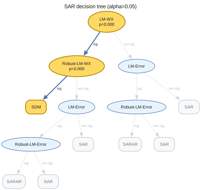
Use Bayesian LM specification tests or spatial block cross-validation instead.
model_diag = SAR(y=y, X=X, W=W)
model_diag.fit(sampler="gibbs", progressbar=False, **COMMON)
model_diag.spatial_diagnostics_decision()
/home/runner/micromamba/envs/test/lib/python3.14/site-packages/neighbayes/_logdet/_jax.py:188: ComplexWarning: Casting complex values to real discards the imaginary part
  W_arr = np.asarray(W, dtype=np.float64)
/home/runner/micromamba/envs/test/lib/python3.14/site-packages/tqdm/auto.py:21: TqdmWarning: IProgress not found. Please update jupyter and ipywidgets. See https://ipywidgets.readthedocs.io/en/stable/user_install.html
  from .autonotebook import tqdm as notebook_tqdm
See also
Supported Models — the block structure, every backend, and all eleven log-determinant methods
Architecture — why conjugacy beats gradients here
How to set priors — the σ² prior is what keeps that block conjugate
How to run Bayesian LM specification tests — choosing which model to fit, before tuning how you fit it
Performance & Profiling — Gibbs-versus-NUTS and backend timings at realistic \(n\)