import geopandas as gpdimport numpy as npimport pandas as pdimport scipyfrom formulaic import Formulafrom geosnap import DataStorefrom geosnap import io as giofrom libpysal.graph import Graphfrom shapely import LineStringfrom spreg import GMM_Error, GM_Lag%load_ext watermark%watermark -a 'eli knaap'
OMP: Info #276: omp_set_nested routine deprecated, please use omp_set_max_active_levels instead.
Author: eli knaap
What if our flows are not independent?
Like any regression, a critical assumption in spatial interaction models is that observations are independent from one another. And like any model using spatial data, the model is misspecified if residuals are spatially autocorrelated (indicating the input data fail the independence criterion). We can use spatial econometric approaches to handle this situation, albeit with some minor modifications because
autocorrelation may come from origins, destinations, or both
we need to approximate the data using a log-linear model instead of proper Poisson
Approaches for estimating spatial lag models are described in LeSage, Fischer, and Scherngell (2007) and LeSage and Pace (2008) while error models are described by Fischer and Griffith (2008), the latter two of which use conventional estimation techniques with specialized \(W\) matrices based on the notion of neighboring origins or neighboring destinations. We explore how to conduct these analyses below. For further background, consult Fischer and Griffith (2008), LeSage, Fischer, and Scherngell (2007), LeSage and Pace (2008), LeSage and Fischer (2010), LeSage and Llano (2013), LeSage (2014), Thomas-Agnan and LeSage (2014), Griffith, Fischer, and LeSage (2017) and Ord (1975).
4.1 Spatial Econometric Models
In the following example we will focus on the spatial interaction specification of two workhorse models in spatial econometrics: the “spatial lag” and “spatial error” models. Following the log-linear specification from the prior section, these are given by
Note there’s a sizeable and growing literature focused on the appropriateness of different estimation techniques for count-based models, particularly in the gravity model context (Manning and Mullahy 2001; Santos Silva and Tenreyro 2010, 2011; Silva and Tenreyro 2006). For the purpose of this workshop it’s sufficient to say that log-linear models induce a certain level of bias–and it’s important to be aware. However flow models also display empirical residual autocorrelation, so nonlinear but nonspatial models also induce bias (and it’s hard to estimate nonlinear spatial models). So here we accept one bias in favor of the other for the sake of demonstration and concern for spatial effects. Consult the literature for a deeper dive.
4.2 Data Preparation
We will follow the same data processing steps as in the previous sections, collecting data for Washington D.C. and converting it into a Graph of flows, then merging with additional data from the Census.
/Users/knaaptime/Dropbox/projects/geosnap/geosnap/io/util.py:273: UserWarning: Unable to find local adjustment year for 2021. Attempting from online data
  warn(
/Users/knaaptime/Dropbox/projects/geosnap/geosnap/io/constructors.py:218: UserWarning: Currency columns unavailable at this resolution; not adjusting for inflation
  warn(
4.3 A Confluence of Graphs
What’s “near” to a flow?
4.3.1 Distance Graph
As with the conventional models in the previous section, we need the distance between each OD pair as a variable for our model. Again we keep only tracts in the dataframe in our flow graph (origins), then get distance between observations with no decay using a Graph
# subset the distance graph by the travel graph (remove destinations we dont need)# but this resets weights to 1dc_dist_adj = dc_dist.intersection(dc_flow_graph).adjacency# update with the old valuesdc_dist_adj.update(dc_dist.adjacency)
/var/folders/j8/5bgcw6hs7cqcbbz48d6bsftw0000gp/T/ipykernel_11551/1114346404.py:6: FutureWarning: Setting an item of incompatible dtype is deprecated and will raise an error in a future version of pandas. Value '[ 673.02448689 1714.42369324 1318.28681649 ... 7734.28131571 2519.49437645
  989.25225739]' has dtype incompatible with int8, please explicitly cast to a compatible dtype first.
  dc_dist_adj.update(dc_dist.adjacency)
now create our dataset using the dense matrix ‘melted’ down into a vector
Now we need to relate the origin and destination observations together. To keep things simple, we consider the standard contiguity graph.
contg = Graph.build_contiguity(dc)
contg
<Graph of 206 nodes and 1060 nonzero edges indexed by
 ['11001000101', '11001000102', '11001000201', '11001000202', '1100100030...]>
Imagine you had a flow that moved from north to south like the map below. The ‘neighborhood’ of this flow might be the tracts surrounding the origin in the north, those surrounding the destination in the south, or a combination thereof.
Make this Notebook Trusted to load map: File -> Trust Notebook
4.3.3 Spatial Graphs for Origin-Destination Flows
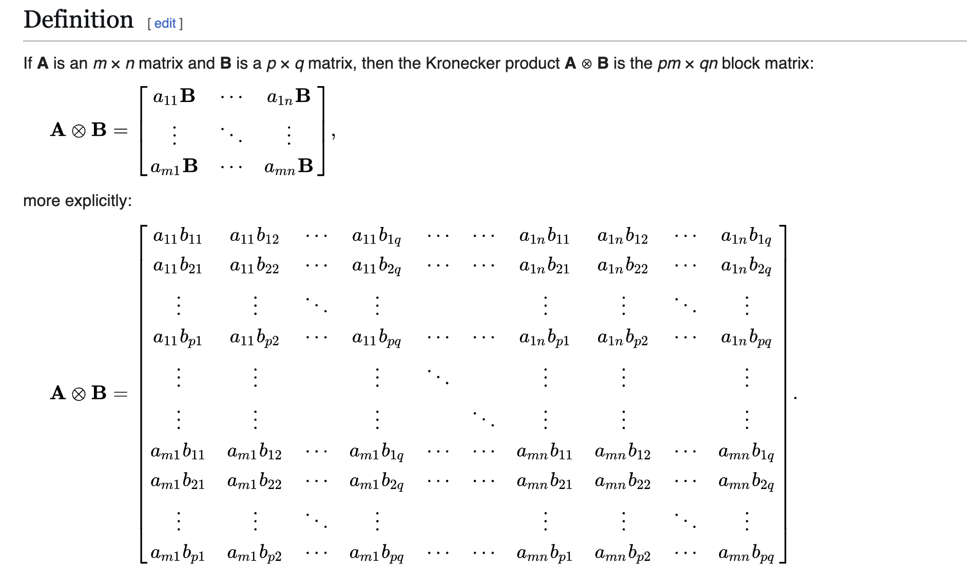
the contg Graph encodes flows as neighbors if the origin tracts share a border. But we need to multiply that graph to get it into the correct dimensions to match our flow data. Following LeSage and Pace (2008) and Fischer and Griffith (2008) we do this via a Kronecker product between our flow and contiguity graphs to create the graph (\(W\)) used in the model.
Kronecker Product
\(G_{flow} \otimes G_{cont}\), where \(\otimes\) is the Kronecker product of the flow graph and contiguity graphs that defines connectivity between origin and destination observations.
In this case observations are neighbors if:
there is a flow between o and d
if o_i shares a border with o_j
three distinct possibilities depending on how the flow graph is ordered
origin-centric weights
destination-centric weights
OD-centric weights (union or sum of oW and dW)
To do this in code, we use scipy to take the Kronecker product of the two Graphs, then re-instantiate a new one.
kg = Graph.from_sparse(scipy.sparse.kron(dc_flow_graph.transform("b").sparse, contg.sparse))
our new graph now as the same length as our observation vector
kg.n
42436
dc_interaction.shape[0]
42436
kg.pct_nonzero
1.3718439929404018
contg.pct_nonzero
2.497879159204449
dc_flow_graph.pct_nonzero
54.9203506456782
since our original Graph has the origin as its focal observation, this is an origin-centric ODW (\(^oW\)), so to get the destination-centric weights (\(^dW\)) you’d do the transpose of the OD matrix (flow graph) first (LeSage and Pace 2008).
row-standardize both origin and destination versions
kg = kg.transform('r')
kgd = kgd.transform('r')
spreg will only treat the Graph as a matrix, so the ordering of the sparse representation is all that matters, not the indices/labels; i.e. the Graph has the correct shape and order even though the indices of the Graph are different than those of the observations
4.4 Main Model Specification
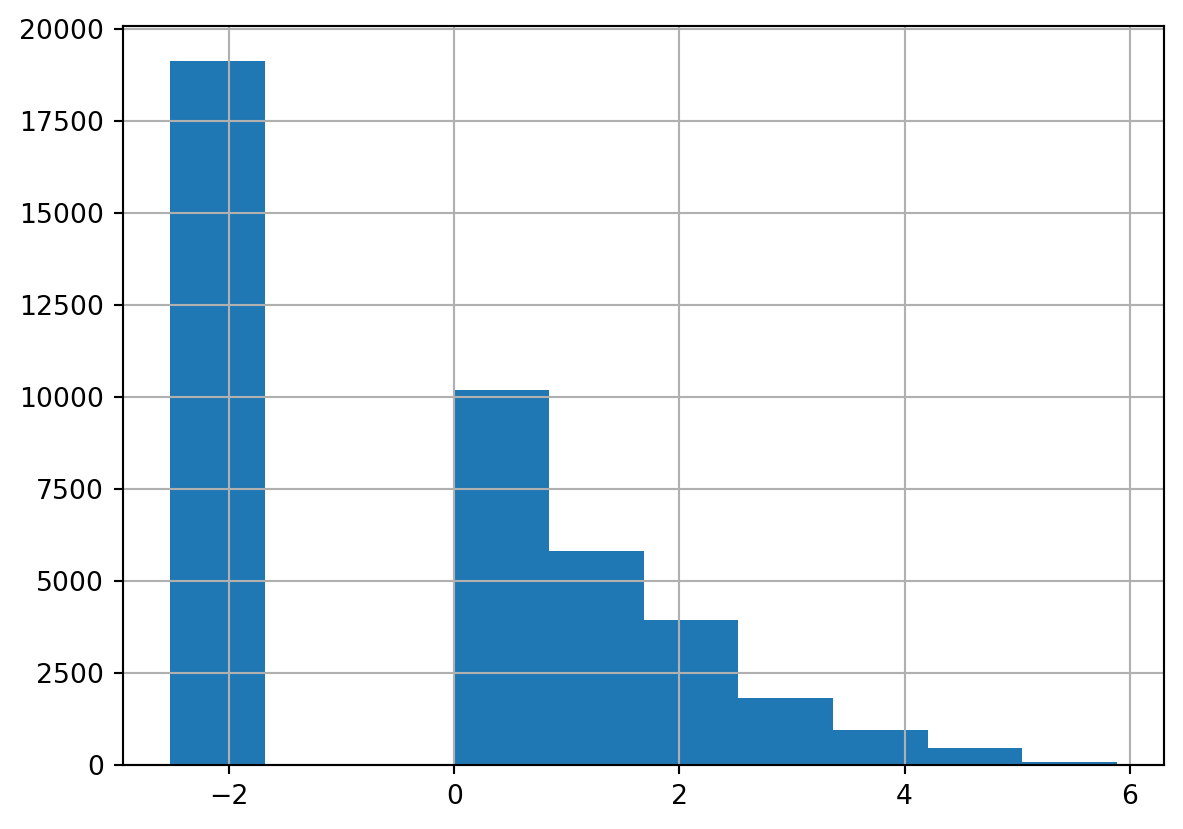
“Note in some cases yij = 0, indicating the absence of flows from i to j. This leads to the so-called zero problem, since the logarithm then is undefined. There are several pragmatic solutions to this problem, with adding a small constant to the zero elements of [yij ] being widely used. Here we added 0.08.” (Fischer and Griffith 2008)
that gives our \(y\) variable a distribution like this
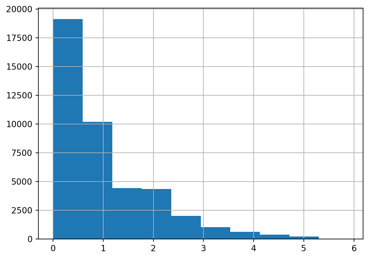
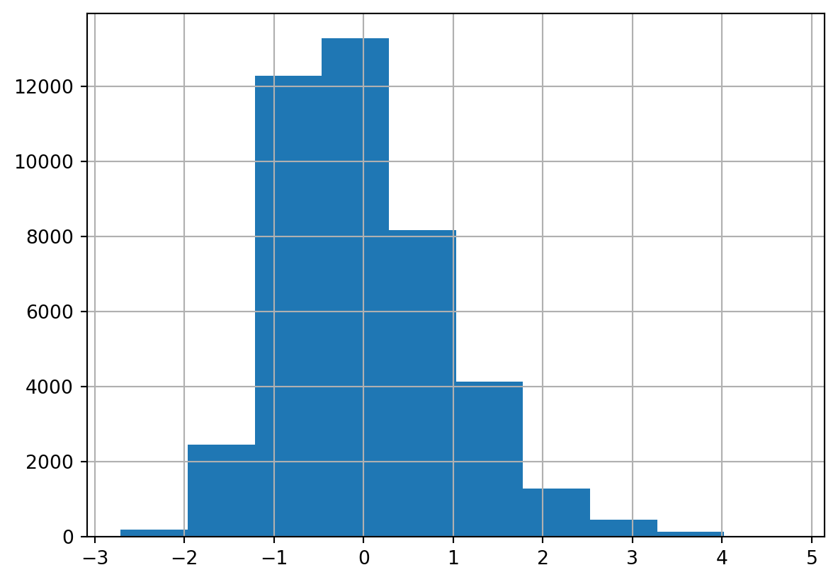
Another common transformation is to add 1 to every observation and take the log of that, i.e. take \(log(x+1)\) (this is setting \(\delta=1\) in Equation 3.2).
dc_interaction.weight.apply(np.log1p).hist()
we specify a log-linear model using formulaic to generate our \(y\) and \(X\) matrices, then pass these to different kinds of spatial econometric models
REGRESSION RESULTS
------------------

SUMMARY OF OUTPUT: SPATIAL TWO STAGE LEAST SQUARES
--------------------------------------------------
Data set            :     unknown
Weights matrix      :     unknown
Dependent Variable  :np.log1p(weight)                Number of Observations:       42436
Mean dependent var  :      0.8921                Number of Variables   :           9
S.D. dependent var  :      1.0715                Degrees of Freedom    :       42427
Pseudo R-squared    :      0.2154
Spatial Pseudo R-squared:  0.1904

------------------------------------------------------------------------------------
            Variable     Coefficient       Std.Error     z-Statistic     Probability
------------------------------------------------------------------------------------
            CONSTANT         1.04565         0.19744         5.29602         0.00000
np.log1p(n_total_pop_origin)         0.21780         0.00992        21.96064         0.00000
np.log1p(median_household_income_origin)         0.01041         0.00996         1.04450         0.29625
np.log1p(p_nonhisp_black_persons_origin)         0.07703         0.00532        14.47604         0.00000
np.log1p(n_total_pop_destination)        -0.20499         0.00996       -20.58275         0.00000
np.log1p(median_household_income_destination)         0.08989         0.00999         9.00130         0.00000
np.log1p(p_nonhisp_black_persons_destination)        -0.20309         0.00571       -35.58426         0.00000
  np.log1p(distance)        -0.16724         0.00519       -32.21315         0.00000
  W_np.log1p(weight)         0.47437         0.01338        35.46370         0.00000
------------------------------------------------------------------------------------
Instrumented: W_np.log1p(weight)
Instruments: W_np.log1p(distance),
             W_np.log1p(median_household_income_destination),
             W_np.log1p(median_household_income_origin),
             W_np.log1p(n_total_pop_destination),
             W_np.log1p(n_total_pop_origin),
             W_np.log1p(p_nonhisp_black_persons_destination),
             W_np.log1p(p_nonhisp_black_persons_origin)
Warning: Variable(s) ['Intercept'] removed for being constant.

DIAGNOSTICS FOR SPATIAL DEPENDENCE
TEST                              DF         VALUE           PROB
Anselin-Kelejian Test             1        375.429           0.0000

SPATIAL LAG MODEL IMPACTS
Impacts computed using the 'simple' method.
            Variable         Direct        Indirect          Total
np.log1p(n_total_pop_origin)         0.2178          0.1966          0.4144
np.log1p(median_household_income_origin)         0.0104          0.0094          0.0198
np.log1p(p_nonhisp_black_persons_origin)         0.0770          0.0695          0.1465
np.log1p(n_total_pop_destination)        -0.2050         -0.1850         -0.3900
np.log1p(median_household_income_destination)         0.0899          0.0811          0.1710
np.log1p(p_nonhisp_black_persons_destination)        -0.2031         -0.1833         -0.3864
  np.log1p(distance)        -0.1672         -0.1509         -0.3182
================================ END OF REPORT =====================================
od_flow_lag.output
var_names
coefficients
std_err
zt_stat
prob
0
CONSTANT
1.045648
0.19744
5.296021
0.0
1
np.log1p(n_total_pop_origin)
0.217802
0.009918
21.960641
0.0
2
np.log1p(median_household_income_origin)
0.010408
0.009965
1.044499
0.296255
3
np.log1p(p_nonhisp_black_persons_origin)
0.07703
0.005321
14.476035
0.0
4
np.log1p(n_total_pop_destination)
-0.20499
0.009959
-20.582747
0.0
5
np.log1p(median_household_income_destination)
0.08989
0.009986
9.001304
0.0
6
np.log1p(p_nonhisp_black_persons_destination)
-0.203087
0.005707
-35.584263
0.0
7
np.log1p(distance)
-0.167245
0.005192
-32.213151
0.0
8
W_np.log1p(weight)
0.474372
0.013376
35.463697
0.0
Instead, we could take the sum of the two graphs, in which case you are neighbors when contiguous with either origin or destination points (same cardinalities as above), but the strength of the weight is 2x if you neighbor both origin and destination.
REGRESSION RESULTS
------------------

SUMMARY OF OUTPUT: SPATIAL TWO STAGE LEAST SQUARES
--------------------------------------------------
Data set            :     unknown
Weights matrix      :     unknown
Dependent Variable  :np.log1p(weight)                Number of Observations:       42436
Mean dependent var  :      0.8921                Number of Variables   :           9
S.D. dependent var  :      1.0715                Degrees of Freedom    :       42427
Pseudo R-squared    :      0.2154
Spatial Pseudo R-squared:  0.1904

------------------------------------------------------------------------------------
            Variable     Coefficient       Std.Error     z-Statistic     Probability
------------------------------------------------------------------------------------
            CONSTANT         1.04565         0.19744         5.29602         0.00000
np.log1p(n_total_pop_origin)         0.21780         0.00992        21.96064         0.00000
np.log1p(median_household_income_origin)         0.01041         0.00996         1.04450         0.29625
np.log1p(p_nonhisp_black_persons_origin)         0.07703         0.00532        14.47604         0.00000
np.log1p(n_total_pop_destination)        -0.20499         0.00996       -20.58275         0.00000
np.log1p(median_household_income_destination)         0.08989         0.00999         9.00130         0.00000
np.log1p(p_nonhisp_black_persons_destination)        -0.20309         0.00571       -35.58426         0.00000
  np.log1p(distance)        -0.16724         0.00519       -32.21315         0.00000
  W_np.log1p(weight)         0.47437         0.01338        35.46370         0.00000
------------------------------------------------------------------------------------
Instrumented: W_np.log1p(weight)
Instruments: W_np.log1p(distance),
             W_np.log1p(median_household_income_destination),
             W_np.log1p(median_household_income_origin),
             W_np.log1p(n_total_pop_destination),
             W_np.log1p(n_total_pop_origin),
             W_np.log1p(p_nonhisp_black_persons_destination),
             W_np.log1p(p_nonhisp_black_persons_origin)
Warning: Variable(s) ['Intercept'] removed for being constant.

DIAGNOSTICS FOR SPATIAL DEPENDENCE
TEST                              DF         VALUE           PROB
Anselin-Kelejian Test             1        375.429           0.0000

SPATIAL LAG MODEL IMPACTS
Impacts computed using the 'simple' method.
            Variable         Direct        Indirect          Total
np.log1p(n_total_pop_origin)         0.2178          0.1966          0.4144
np.log1p(median_household_income_origin)         0.0104          0.0094          0.0198
np.log1p(p_nonhisp_black_persons_origin)         0.0770          0.0695          0.1465
np.log1p(n_total_pop_destination)        -0.2050         -0.1850         -0.3900
np.log1p(median_household_income_destination)         0.0899          0.0811          0.1710
np.log1p(p_nonhisp_black_persons_destination)        -0.2031         -0.1833         -0.3864
  np.log1p(distance)        -0.1672         -0.1509         -0.3182
================================ END OF REPORT =====================================
od_flow_lag.output
var_names
coefficients
std_err
zt_stat
prob
0
CONSTANT
1.045648
0.19744
5.296021
0.0
1
np.log1p(n_total_pop_origin)
0.217802
0.009918
21.960641
0.0
2
np.log1p(median_household_income_origin)
0.010408
0.009965
1.044499
0.296255
3
np.log1p(p_nonhisp_black_persons_origin)
0.07703
0.005321
14.476035
0.0
4
np.log1p(n_total_pop_destination)
-0.20499
0.009959
-20.582747
0.0
5
np.log1p(median_household_income_destination)
0.08989
0.009986
9.001304
0.0
6
np.log1p(p_nonhisp_black_persons_destination)
-0.203087
0.005707
-35.584263
0.0
7
np.log1p(distance)
-0.167245
0.005192
-32.213151
0.0
8
W_np.log1p(weight)
0.474372
0.013376
35.463697
0.0
4.6 Spatial Error
the error models take a really long time to estimate
4.6.1 Origin-Centric
flow_error_origin = GMM_Error(y=y, x=x, w=kg)
print(flow_error_origin.summary)
REGRESSION RESULTS
------------------

SUMMARY OF OUTPUT: GM SPATIALLY WEIGHTED LEAST SQUARES (HET)
------------------------------------------------------------
Data set            :     unknown
Weights matrix      :     unknown
Dependent Variable  :np.log1p(weight)                Number of Observations:       42436
Mean dependent var  :      0.8921                Number of Variables   :           8
S.D. dependent var  :      1.0715                Degrees of Freedom    :       42428
Pseudo R-squared    :      0.1715
N. of iterations    :           1                Step1c computed       :          No

------------------------------------------------------------------------------------
            Variable     Coefficient       Std.Error     z-Statistic     Probability
------------------------------------------------------------------------------------
            CONSTANT         0.56346         0.20423         2.75895         0.00580
np.log1p(n_total_pop_origin)         0.21456         0.00891        24.06762         0.00000
np.log1p(median_household_income_origin)         0.00795         0.00984         0.80835         0.41889
np.log1p(p_nonhisp_black_persons_origin)         0.07338         0.00519        14.13295         0.00000
np.log1p(n_total_pop_destination)        -0.15311         0.01360       -11.25810         0.00000
np.log1p(median_household_income_destination)         0.14984         0.01078        13.89702         0.00000
np.log1p(p_nonhisp_black_persons_destination)        -0.22535         0.00724       -31.13522         0.00000
  np.log1p(distance)        -0.17330         0.00611       -28.36196         0.00000
              lambda         0.43320         0.00102       425.12538         0.00000
------------------------------------------------------------------------------------
Warning: Variable(s) ['Intercept'] removed for being constant.
================================ END OF REPORT =====================================
flow_error_origin.output
var_names
coefficients
std_err
zt_stat
prob
0
CONSTANT
0.563463
0.204231
2.758949
0.005799
1
np.log1p(n_total_pop_origin)
0.214562
0.008915
24.06762
0.0
2
np.log1p(median_household_income_origin)
0.007952
0.009837
0.808354
0.418887
3
np.log1p(p_nonhisp_black_persons_origin)
0.073376
0.005192
14.132946
0.0
4
np.log1p(n_total_pop_destination)
-0.153111
0.0136
-11.258098
0.0
5
np.log1p(median_household_income_destination)
0.14984
0.010782
13.89702
0.0
6
np.log1p(p_nonhisp_black_persons_destination)
-0.225354
0.007238
-31.135217
0.0
7
np.log1p(distance)
-0.173299
0.00611
-28.361959
0.0
8
lambda
0.433203
0.001019
425.125382
0.0
4.6.2 Destination-centric
flow_error_dest = GMM_Error(y=y, x=x, w=kgd)
print(flow_error_dest.summary)
REGRESSION RESULTS
------------------

SUMMARY OF OUTPUT: GM SPATIALLY WEIGHTED LEAST SQUARES (HET)
------------------------------------------------------------
Data set            :     unknown
Weights matrix      :     unknown
Dependent Variable  :np.log1p(weight)                Number of Observations:       42436
Mean dependent var  :      0.8921                Number of Variables   :           8
S.D. dependent var  :      1.0715                Degrees of Freedom    :       42428
Pseudo R-squared    :      0.1715
N. of iterations    :           1                Step1c computed       :          No

------------------------------------------------------------------------------------
            Variable     Coefficient       Std.Error     z-Statistic     Probability
------------------------------------------------------------------------------------
            CONSTANT         0.56128         0.20497         2.73832         0.00618
np.log1p(n_total_pop_origin)         0.21696         0.00897        24.19122         0.00000
np.log1p(median_household_income_origin)         0.00546         0.01003         0.54423         0.58628
np.log1p(p_nonhisp_black_persons_origin)         0.07677         0.00523        14.68281         0.00000
np.log1p(n_total_pop_destination)        -0.15614         0.01318       -11.84381         0.00000
np.log1p(median_household_income_destination)         0.15218         0.01086        14.00732         0.00000
np.log1p(p_nonhisp_black_persons_destination)        -0.22997         0.00737       -31.19187         0.00000
  np.log1p(distance)        -0.17405         0.00615       -28.27823         0.00000
              lambda         0.50877         0.00117       434.08837         0.00000
------------------------------------------------------------------------------------
Warning: Variable(s) ['Intercept'] removed for being constant.
================================ END OF REPORT =====================================
flow_error_dest.output
var_names
coefficients
std_err
zt_stat
prob
0
CONSTANT
0.561276
0.204971
2.73832
0.006175
1
np.log1p(n_total_pop_origin)
0.216964
0.008969
24.191224
0.0
2
np.log1p(median_household_income_origin)
0.005457
0.010026
0.544231
0.586282
3
np.log1p(p_nonhisp_black_persons_origin)
0.076774
0.005229
14.682813
0.0
4
np.log1p(n_total_pop_destination)
-0.156139
0.013183
-11.843813
0.0
5
np.log1p(median_household_income_destination)
0.152175
0.010864
14.00732
0.0
6
np.log1p(p_nonhisp_black_persons_destination)
-0.229974
0.007373
-31.191871
0.0
7
np.log1p(distance)
-0.174048
0.006155
-28.278234
0.0
8
lambda
0.50877
0.001172
434.088366
0.0
4.6.3 OD-Centric
flow_error_od = GMM_Error(y=y, x=x, w=kg_od)
print(flow_error_od.summary)
REGRESSION RESULTS
------------------

SUMMARY OF OUTPUT: GM SPATIALLY WEIGHTED LEAST SQUARES (HET)
------------------------------------------------------------
Data set            :     unknown
Weights matrix      :     unknown
Dependent Variable  :np.log1p(weight)                Number of Observations:       42436
Mean dependent var  :      0.8921                Number of Variables   :           8
S.D. dependent var  :      1.0715                Degrees of Freedom    :       42428
Pseudo R-squared    :      0.1715
N. of iterations    :           1                Step1c computed       :          No

------------------------------------------------------------------------------------
            Variable     Coefficient       Std.Error     z-Statistic     Probability
------------------------------------------------------------------------------------
            CONSTANT         0.56353         0.20413         2.76064         0.00577
np.log1p(n_total_pop_origin)         0.21591         0.00891        24.23514         0.00000
np.log1p(median_household_income_origin)         0.00649         0.00986         0.65821         0.51041
np.log1p(p_nonhisp_black_persons_origin)         0.07679         0.00515        14.90760         0.00000
np.log1p(n_total_pop_destination)        -0.15462         0.01346       -11.48887         0.00000
np.log1p(median_household_income_destination)         0.15089         0.01081        13.95301         0.00000
np.log1p(p_nonhisp_black_persons_destination)        -0.22738         0.00729       -31.21079         0.00000
  np.log1p(distance)        -0.17427         0.00611       -28.50641         0.00000
              lambda         0.45731         0.00098       468.34007         0.00000
------------------------------------------------------------------------------------
Warning: Variable(s) ['Intercept'] removed for being constant.
================================ END OF REPORT =====================================
flow_error_od.output
var_names
coefficients
std_err
zt_stat
prob
0
CONSTANT
0.563534
0.204132
2.760642
0.005769
1
np.log1p(n_total_pop_origin)
0.215913
0.008909
24.235136
0.0
2
np.log1p(median_household_income_origin)
0.006487
0.009855
0.658206
0.510406
3
np.log1p(p_nonhisp_black_persons_origin)
0.076789
0.005151
14.907596
0.0
4
np.log1p(n_total_pop_destination)
-0.154617
0.013458
-11.488873
0.0
5
np.log1p(median_household_income_destination)
0.15089
0.010814
13.953006
0.0
6
np.log1p(p_nonhisp_black_persons_destination)
-0.227383
0.007285
-31.210786
0.0
7
np.log1p(distance)
-0.174273
0.006113
-28.506414
0.0
8
lambda
0.457305
0.000976
468.340074
0.0
Note
As an alternative to the spatial econometric specifications illustrated above, Liao and Oshan (2025) recently described a different model that incorporates the “intervening opportunities” and “competing destinations” frameworks discussed in the spatial interaction literature by incorporating two additional terms \(A_i\) and \(A_j\) which represent accessibility measures at the origin and destination locations, respectively. In spatial econometric parlance, this approach is equivalent to a spatial lag of X (SLX) model with terms that include both origin-centric and destination-centric lagged X variables (LeSage and Fischer 2016).
4.7 References
Fischer, Manfred M., and Daniel A. Griffith. 2008. “Modeling Spatial Autocorrelation in Spatial Interaction Data: An Application to Patent Citation Data in the European Union.”Journal of Regional Science 48 (5): 969–89. https://doi.org/10.1111/j.1467-9787.2008.00572.x.
Griffith, Daniel A., Manfred M. Fischer, and James LeSage. 2017. “The Spatial Autocorrelation Problem in Spatial Interaction Modelling: A Comparison of Two Common Solutions.”Letters in Spatial and Resource Sciences 10 (1): 75–86. https://doi.org/10.1007/s12076-016-0172-8.
LeSage, James P. 2014. “What Regional Scientists Need to Know About Spatial Econometrics.”SSRN Electronic Journal. https://doi.org/10.2139/ssrn.2420725.
LeSage, James P., and Manfred M. Fischer. 2010. “Spatial Econometric Methods for Modeling Origin-Destination Flows.” In Handbook of Applied Spatial Analysis: Software Tools, Methods and Applications, edited by Manfred M. Fischer and Arthur Getis, 409–33. Berlin, Heidelberg: Springer. https://doi.org/10.1007/978-3-642-03647-7_20.
———. 2016. “Spatial Regression-Based Model Specifications for Exogenous and Endogenous Spatial Interaction.” In Spatial Econometric Interaction Modelling, edited by Roberto Patuelli and Giuseppe Arbia, 15–36. Cham: Springer International Publishing. https://doi.org/10.1007/978-3-319-30196-9_2.
LeSage, James P., Manfred M. Fischer, and Thomas Scherngell. 2007. “Knowledge Spillovers Across Europe: Evidence from a Poisson Spatial Interaction Model with Spatial Effects.”Papers in Regional Science 86 (3): 393–421. https://doi.org/10.1111/j.1435-5957.2007.00125.x.
LeSage, James P., and Carlos Llano. 2013. “A Spatial Interaction Model with Spatially Structured Origin and Destination Effects.”Journal of Geographical Systems 15 (3): 265–89. https://doi.org/10.1007/s10109-013-0181-8.
LeSage, James P., and R Kelley Pace. 2008. “Spatial Econometric Modeling Of Origin-Destination Flows.”Journal of Regional Science 48 (5): 941–67. https://doi.org/10.1111/j.1467-9787.2008.00573.x.
Liao, Mengyu, and Taylor M. Oshan. 2025. “A Data‐Driven Approach to Spatial Interaction Models of Migration: Integrating and Refining the Theories of Competing Destinations and Intervening Opportunities.”Geographical Analysis, March. https://doi.org/10.1111/gean.70001.
Manning, Willard G, and John Mullahy. 2001. “Estimating Log Models: To Transform or Not to Transform?”Journal of Health Economics 20 (4): 461–94. https://doi.org/10.1016/S0167-6296(01)00086-8.
Ord, J K. 1975. “Estimation Methods for Models of Spatial Interaction.”Journal of the American Statistical Association 70 (349): 120–26. https://doi.org/10.1080/01621459.1975.10480272.
Santos Silva, J. M. C., and Silvana Tenreyro. 2010. “On the Existence of the Maximum Likelihood Estimates in Poisson Regression.”Economics Letters 107 (2): 310–12. https://doi.org/10.1016/j.econlet.2010.02.020.
———. 2011. “Further Simulation Evidence on the Performance of the Poisson Pseudo-Maximum Likelihood Estimator.”Economics Letters 112 (2): 220–22. https://doi.org/10.1016/j.econlet.2011.05.008.
Thomas-Agnan, Christine, and James P. LeSage. 2014. “Spatial Econometric OD-Flow Models.” In Handbook of Regional Science, edited by Manfred M. Fischer and Peter Nijkamp, 1653–73. Berlin, Heidelberg: Springer Berlin Heidelberg. https://doi.org/10.1007/978-3-642-23430-9_87.