Cross-Sectional Model Comparison: neighbayes vs spreg
Columbus example
This notebook compares equivalent cross-sectional models between neighbayes and spreg on a real example dataset from the PySAL/spreg ecosystem.
The dependent variable is HOVAL, with INC and CRIME used as explanatory variables.
Model mapping used:
SLX(neighbayes) vsspreg.OLS(slx_lags=1)SAR(neighbayes) vsspreg.GM_LagSEM(neighbayes) vsspreg.GM_ErrorSDM(neighbayes) vsspreg.GM_Lag(slx_lags=1, w_lags=2)SDEM(neighbayes) vsspreg.GM_Error(slx_lags=1)
Dataset: Columbus neighborhood data from libpysal.examples.
import geopandas as gpd
import libpysal
import numpy as np
import pandas as pd
import spreg
from IPython.display import display
from spreg.sputils import _sp_effects, spmultiplier

from neighbayes.models import SAR, SDEM, SDM, SEM, SLX
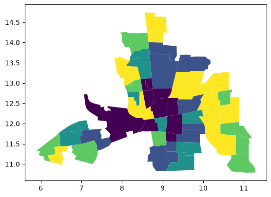
columbus = gpd.read_file(libpysal.examples.get_path("columbus.shp"))
columbus.plot("HOVAL", scheme="quantiles")
<Axes: >
w = libpysal.graph.Graph.build_contiguity(columbus).transform("r")
y = columbus.HOVAL.values
X = columbus[["INC", "CRIME"]]

spreg_results = {
    "SLX": spreg.OLS(y, X, w=w, slx_lags=1, name_y="HOVAL", name_x=["INC", "CRIME"]),
    "SAR": spreg.ML_Lag(y, X, w=w, name_y="HOVAL", name_x=["INC", "CRIME"]),
    "SEM": spreg.ML_Error(y, X, w=w, name_y="HOVAL", name_x=["INC", "CRIME"]),
    "SDM": spreg.ML_Lag(
        y, X, w=w, slx_lags=1, w_lags=2, name_y="HOVAL", name_x=["INC", "CRIME"]
    ),
    "SDEM": spreg.GM_Error(
        y, X, w=w, slx_lags=1, name_y="HOVAL", name_x=["INC", "CRIME"]
    ),
}

spec = "HOVAL ~  1 + INC + CRIME"
sample_kwargs = dict(draws=1000, tune=1000, chains=4, random_seed=42, progressbar=False)
bayes_models = {
    "SLX": SLX(spec, data=columbus, W=w),
    "SAR": SAR(spec, data=columbus, W=w),
    "SEM": SEM(spec, data=columbus, W=w),
    "SDM": SDM(spec, data=columbus, W=w),
    "SDEM": SDEM(spec, data=columbus, W=w),
}
bayes_idata = {name: model.fit(**sample_kwargs) for name, model in bayes_models.items()}
ML_Lag
ML_Error
ML_Lag
GM_Error
/home/runner/micromamba/envs/test/lib/python3.14/site-packages/spreg/diagnostics.py:620: ComplexWarning: Casting complex values to real discards the imaginary part
  ci_result = sqrt(max_eigval / min_eigval)
/home/runner/micromamba/envs/test/lib/python3.14/site-packages/spreg/ml_error.py:184: RuntimeWarning: Method 'bounded' does not support relative tolerance in x; defaulting to absolute tolerance.
  res = minimize_scalar(
Initializing NUTS using jitter+adapt_diag...
Multiprocess sampling (4 chains in 2 jobs)
NUTS: [beta, sigma2]
Sampling 4 chains for 1_000 tune and 1_000 draw iterations (4_000 + 4_000 draws total) took 16 seconds.
/home/runner/micromamba/envs/test/lib/python3.14/site-packages/neighbayes/_logdet/_jax.py:188: ComplexWarning: Casting complex values to real discards the imaginary part
  W_arr = np.asarray(W, dtype=np.float64)
bayes_models["SAR"].summary()
| mean | sd | hdi_3% | hdi_97% | mcse_mean | mcse_sd | ess_bulk | ess_tail | r_hat | |
|---|---|---|---|---|---|---|---|---|---|
| rho | 0.212 | 0.167 | -0.100 | 0.532 | 0.003 | 0.003 | 4119.0 | 3042.0 | 1.0 |
| sigma | 15.032 | 1.531 | 12.134 | 17.822 | 0.026 | 0.019 | 3534.0 | 3797.0 | 1.0 |
| sigma2 | 228.293 | 47.386 | 145.507 | 315.788 | 0.789 | 0.691 | 3534.0 | 3797.0 | 1.0 |
| Intercept | 37.939 | 13.899 | 12.610 | 64.089 | 0.225 | 0.161 | 3802.0 | 3434.0 | 1.0 |
| INC | 0.574 | 0.528 | -0.422 | 1.522 | 0.009 | 0.006 | 3748.0 | 4057.0 | 1.0 |
| CRIME | -0.454 | 0.177 | -0.768 | -0.101 | 0.003 | 0.002 | 3850.0 | 3920.0 | 1.0 |
Sampler adequacy for \(\rho\)
Before trusting the SAR posterior summary above, verify that the spatial parameter \(\rho\) has been sampled efficiently. Wolf, Anselin & Arribas-Bel (2018) [Wolf et al., 2018] show that \(\rho\) tends to mix slowly, so a chain that converges in mean can still under-cover the tails by 10–12 %.
from neighbayes.diagnostics import spatial_mcmc_diagnostic

spatial_mcmc_diagnostic(bayes_models["SAR"], emit_warnings=False).to_frame()
| ess_bulk | ess_tail | r_hat | mcse_mean | yield_pct | hpdi_drift_pct | adequate | |
|---|---|---|---|---|---|---|---|
| parameter | |||||||
| rho | 4118.821751 | 3041.960166 | 0.999832 | 0.00262 | 102.970544 | 0.07253 | True |
print(spreg_results["SAR"].summary)
REGRESSION RESULTS
------------------

SUMMARY OF OUTPUT: MAXIMUM LIKELIHOOD SPATIAL LAG (METHOD = FULL)
------------------------------------------------------------------------------------
Data set            :     unknown
Weights matrix      :     unknown
Dependent Variable  :       HOVAL                Number of Observations:          49
Mean dependent var  :     38.4362                Number of Variables   :           4
S.D. dependent var  :     18.4661                Degrees of Freedom    :          45
Pseudo R-squared    :      0.3826
Spatial Pseudo R-squared:  0.3271
Log likelihood      :   -200.4394
Sigma-square ML     :    206.3220                Akaike info criterion :     408.879
S.E of regression   :     14.3639                Schwarz criterion     :     416.446

------------------------------------------------------------------------------------
            Variable     Coefficient       Std.Error     z-Statistic     Probability
------------------------------------------------------------------------------------
            CONSTANT        37.26813        13.94565         2.67238         0.00753
                 INC         0.56316         0.51316         1.09742         0.27246
               CRIME        -0.45102         0.17770        -2.53815         0.01114
             W_HOVAL         0.23063         0.15496         1.48836         0.13666
------------------------------------------------------------------------------------

SPATIAL LAG MODEL IMPACTS
Impacts computed using the 'simple' method.
            Variable         Direct        Indirect          Total
                 INC         0.5632          0.1688          0.7320
               CRIME        -0.4510         -0.1352         -0.5862
================================ END OF REPORT =====================================
def extract_spreg_params(model):
    names = list(getattr(model, "name_x", []))
    betas = np.asarray(model.betas).flatten()
    if len(betas) == len(names) + 1 and type(model).__name__ == "GM_Lag":
        names = names + ["rho"]
    if len(names) != len(betas):
        names = [f"param_{i}" for i in range(len(betas))]
    return pd.Series(betas, index=names, dtype=float)


def extract_neighbayes_params(model_name, model, idata):
    out = {}
    beta_mean = idata.posterior["beta"].mean(("chain", "draw")).values
    beta_names = (
        model._beta_names()
        if model_name in {"SLX", "SDM", "SDEM"}
        else list(model._feature_names)
    )
    for name, val in zip(beta_names, beta_mean):
        out[name] = float(val)
    if model_name in {"SAR", "SDM"}:
        out["rho"] = float(idata.posterior["rho"].mean())
    if model_name in {"SEM", "SDEM"}:
        out["lambda"] = float(idata.posterior["lam"].mean())
    harmonized = {}
    for k, v in out.items():
        key = k.replace("W*", "W_")
        if key.lower() == "intercept":
            key = "CONSTANT"
        harmonized[key] = v
    return pd.Series(harmonized, dtype=float)


def bayes_effects_df(model):
    eff = model.spatial_effects()
    # spatial_effects() returns a DataFrame indexed by feature names
    return pd.DataFrame(
        {
            "feature": eff.index.tolist(),
            "direct_neighbayes": eff["direct"].values,
            "indirect_neighbayes": eff["indirect"].values,
            "total_neighbayes": eff["total"].values,
        }
    )


def spreg_effects_df(model_name, sp_model):
    if model_name == "SEM":
        # SEM has no spatial multiplier on the systematic component,
        # so direct = coefficient, indirect = 0, total = coefficient.
        # neighbayes excludes the intercept from effects, so we
        # only compare non-constant covariates here.
        sp_params = extract_spreg_params(sp_model)
        features = [f for f in ["INC", "CRIME"] if f in sp_params.index]
        return pd.DataFrame(
            {
                "feature": features,
                "direct_spreg": [float(sp_params[f]) for f in features],
                "indirect_spreg": [0.0 for _ in features],
                "total_spreg": [float(sp_params[f]) for f in features],
            }
        )

    output = sp_model.output.copy()
    output["regime"] = "global"

    def classify_var(var_name):
        if var_name == "CONSTANT":
            return "o"
        if var_name in {"lambda", "W_HOVAL"}:
            return "rho"
        if var_name.startswith("W_"):
            return "wx"
        return "x"

    output["var_type"] = output["var_names"].map(classify_var)
    sp_model.output = output

    vars_x = output.query("var_type == 'x'")
    rho = (
        float(np.squeeze(getattr(sp_model, "rho", 0.0)))
        if hasattr(sp_model, "rho")
        else 0.0
    )
    multipliers = spmultiplier(w, rho)
    slx_lags = getattr(sp_model, "slx_lags", 0) or (
        1 if model_name in {"SLX", "SDEM"} else 0
    )
    slx_vars = getattr(sp_model, "slx_vars", None)
    if slx_vars is None:
        slx_vars = "All"

    total_spreg, direct_spreg, indirect_spreg = _sp_effects(
        sp_model,
        vars_x,
        multipliers,
        slx_lags=slx_lags,
        slx_vars=slx_vars,
    )

    return pd.DataFrame(
        {
            "feature": vars_x["var_names"].tolist(),
            "direct_spreg": np.asarray(direct_spreg).flatten(),
            "indirect_spreg": np.asarray(indirect_spreg).flatten(),
            "total_spreg": np.asarray(total_spreg).flatten(),
        }
    )


coef_rows = []
effect_tables = {}

for model_name in ["SLX", "SAR", "SEM", "SDM", "SDEM"]:
    sp = extract_spreg_params(spreg_results[model_name])
    by = extract_neighbayes_params(
        model_name, bayes_models[model_name], bayes_idata[model_name]
    )

    common = sorted(set(sp.index).intersection(set(by.index)))
    for param in common:
        coef_rows.append(
            {
                "model": model_name,
                "parameter": param,
                "neighbayes_posterior_mean": by[param],
                "spreg_estimate": sp[param],
                "difference": by[param] - sp[param],
            }
        )

    beff = bayes_effects_df(bayes_models[model_name]).copy()
    seff = spreg_effects_df(model_name, spreg_results[model_name]).copy()
    merged = beff.merge(seff, on="feature", how="inner")
    if not merged.empty:
        merged["direct_difference"] = (
            merged["direct_neighbayes"] - merged["direct_spreg"]
        )
        merged["indirect_difference"] = (
            merged["indirect_neighbayes"] - merged["indirect_spreg"]
        )
        merged["total_difference"] = merged["total_neighbayes"] - merged["total_spreg"]
        merged.insert(0, "model", model_name)
    effect_tables[model_name] = merged

comparison = (
    pd.DataFrame(coef_rows).sort_values(["model", "parameter"]).reset_index(drop=True)
)
spatial_effects_comparison = pd.concat(
    [tbl for tbl in effect_tables.values() if not tbl.empty],
    ignore_index=True,
)
Coefficient comparison
display(comparison)
| model | parameter | neighbayes_posterior_mean | spreg_estimate | difference | |
|---|---|---|---|---|---|
| 0 | SAR | CONSTANT | 37.938906 | 37.268135 | 0.670771 |
| 1 | SAR | CRIME | -0.453989 | -0.451020 | -0.002969 |
| 2 | SAR | INC | 0.573664 | 0.563156 | 0.010509 |
| 3 | SDEM | CONSTANT | 32.107988 | 29.460538 | 2.647450 |
| 4 | SDEM | CRIME | -0.583494 | -0.575430 | -0.008064 |
| 5 | SDEM | INC | 0.839808 | 0.820920 | 0.018889 |
| 6 | SDEM | W_CRIME | 0.242009 | 0.300693 | -0.058685 |
| 7 | SDEM | W_INC | 0.451883 | 0.478086 | -0.026203 |
| 8 | SDEM | lambda | 0.432330 | 0.358330 | 0.074000 |
| 9 | SDM | CONSTANT | 23.621707 | 17.045361 | 6.576346 |
| 10 | SDM | CRIME | -0.609352 | -0.608430 | -0.000922 |
| 11 | SDM | INC | 0.762524 | 0.803686 | -0.041162 |
| 12 | SDM | W_CRIME | 0.399872 | 0.475451 | -0.075580 |
| 13 | SDM | W_INC | -0.072790 | 0.042213 | -0.115003 |
| 14 | SEM | CONSTANT | 47.234057 | 48.008252 | -0.774195 |
| 15 | SEM | CRIME | -0.555294 | -0.559458 | 0.004164 |
| 16 | SEM | INC | 0.756096 | 0.711532 | 0.044564 |
| 17 | SEM | lambda | 0.415846 | 0.390499 | 0.025348 |
| 18 | SLX | CONSTANT | 29.978742 | 27.727885 | 2.250857 |
| 19 | SLX | CRIME | -0.579939 | -0.590675 | 0.010737 |
| 20 | SLX | INC | 0.745974 | 0.742442 | 0.003532 |
| 21 | SLX | W_CRIME | 0.354822 | 0.390156 | -0.035335 |
| 22 | SLX | W_INC | 0.390795 | 0.486179 | -0.095384 |
Direct/Indirect/Total effects comparison
display(spatial_effects_comparison)
| model | feature | direct_neighbayes | indirect_neighbayes | total_neighbayes | direct_spreg | indirect_spreg | total_spreg | direct_difference | indirect_difference | total_difference | |
|---|---|---|---|---|---|---|---|---|---|---|---|
| 0 | SLX | INC | 0.745974 | 0.390795 | 1.136769 | 0.742442 | 0.486179 | 1.228621 | 0.003532 | -0.095384 | -0.091852 |
| 1 | SLX | CRIME | -0.579939 | 0.354822 | -0.225117 | -0.590675 | 0.390156 | -0.200519 | 0.010737 | -0.035335 | -0.024598 |
| 2 | SAR | INC | 0.586206 | 0.176688 | 0.762894 | 0.563156 | 0.168814 | 0.731970 | 0.023050 | 0.007874 | 0.030924 |
| 3 | SAR | CRIME | -0.464093 | -0.141969 | -0.606061 | -0.451020 | -0.135200 | -0.586219 | -0.013073 | -0.006769 | -0.019842 |
| 4 | SEM | INC | 0.756096 | 0.000000 | 0.756096 | 0.711532 | 0.000000 | 0.711532 | 0.044564 | 0.000000 | 0.044564 |
| 5 | SEM | CRIME | -0.555294 | 0.000000 | -0.555294 | -0.559458 | 0.000000 | -0.559458 | 0.004164 | 0.000000 | 0.004164 |
| 6 | SDM | INC | 0.788745 | 0.304948 | 1.093693 | 0.803686 | 0.523510 | 1.327196 | -0.014941 | -0.218562 | -0.233503 |
| 7 | SDM | CRIME | -0.595859 | 0.260551 | -0.335309 | -0.608430 | 0.399790 | -0.208640 | 0.012570 | -0.139239 | -0.126669 |
| 8 | SDEM | INC | 0.839808 | 0.451883 | 1.291691 | 0.820920 | 0.478086 | 1.299005 | 0.018889 | -0.026203 | -0.007314 |
| 9 | SDEM | CRIME | -0.583494 | 0.242009 | -0.341485 | -0.575430 | 0.300693 | -0.274737 | -0.008064 | -0.058685 | -0.066748 |
neighbayes uses Bayesian inference while spreg reports frequentist point estimates, so exact equality is not expected. The coefficient and effects tables are intended to verify directional and numerical agreement under matched model formulas with HOVAL as the dependent variable.
For effects, this notebook now uses spreg’s own spatial-impact utilities: spreg.sputils.spmultiplier and spreg.sputils._sp_effects. SEM is the one exception, since it has no spatial multiplier on the systematic component and therefore uses direct = coefficient, indirect = 0, total = coefficient.
Note on intercept exclusion: neighbayes excludes the intercept from spatial effects for all model types, since the intercept has no meaningful spatial impact interpretation. This is consistent with spreg’s _sp_effects, which also excludes the constant (CONSTANT) from its impact calculations.
Example: Synthetic Data on a 30x30 Grid
This example demonstrates how to generate synthetic spatial data on a 30x30 regular grid, construct a spatial weights matrix, and fit a cross-sectional spatial regression model using the neighbayes package.
from neighbayes import dgp
from neighbayes.models import SAR

# Set random seed for reproducibility
np.random.seed(42)

# True parameters
beta_true = np.array([1.0, -1.0])
rho_true = 0.5
sigma_true = 1.0

gdf = dgp.simulate_sar(
    n=40,
    beta=beta_true,
    rho=rho_true,
    sigma=sigma_true,
    create_gdf=True,
    contiguity="queen",
)

w = libpysal.graph.Graph.build_contiguity(gdf, rook=False).transform("r")

# Fit SAR model
model = SAR("y ~ X_1", W=w, data=gdf)
res = model.fit()

model.summary()
Gibbs sampling (sar): 4 chains for 1,000 tune and 2,000 draw iterations (4 x 3,000 = 12,000 draws total)
/home/runner/micromamba/envs/test/lib/python3.14/site-packages/rich/live.py:260: UserWarning: install "ipywidgets"
for Jupyter support
  warnings.warn('install "ipywidgets" for Jupyter support')
Sampling took 4s (3,407 draws/s)
| mean | sd | hdi_3% | hdi_97% | mcse_mean | mcse_sd | ess_bulk | ess_tail | r_hat | |
|---|---|---|---|---|---|---|---|---|---|
| rho | 0.512 | 0.027 | 0.461 | 0.565 | 0.000 | 0.000 | 7693.0 | 5844.0 | 1.0 |
| sigma | 1.038 | 0.019 | 1.004 | 1.074 | 0.000 | 0.000 | 7936.0 | 7660.0 | 1.0 |
| sigma2 | 1.078 | 0.038 | 1.008 | 1.154 | 0.000 | 0.000 | 7936.0 | 7660.0 | 1.0 |
| Intercept | 0.951 | 0.059 | 0.845 | 1.067 | 0.001 | 0.001 | 7714.0 | 6495.0 | 1.0 |
| X_1 | -1.039 | 0.026 | -1.089 | -0.991 | 0.000 | 0.000 | 8210.0 | 7728.0 | 1.0 |
model.spatial_effects()
| direct | direct_ci_lower | direct_ci_upper | direct_pvalue | indirect | indirect_ci_lower | indirect_ci_upper | indirect_pvalue | total | total_ci_lower | total_ci_upper | total_pvalue | |
|---|---|---|---|---|---|---|---|---|---|---|---|---|
| variable | ||||||||||||
| X_1 | -1.088809 | -1.143583 | -1.034024 | 0.0 | -1.045492 | -1.297881 | -0.835712 | 0.0 | -2.134301 | -2.41185 | -1.895391 | 0.0 |
sim_spreg = spreg.GM_Lag(
    gdf["y"],
    gdf["X_1"],
    w=w,
)
GM_Lag
print(sim_spreg.summary)
REGRESSION RESULTS
------------------

SUMMARY OF OUTPUT: SPATIAL TWO STAGE LEAST SQUARES
------------------------------------------------------------------------------------
Data set            :     unknown
Weights matrix      :     unknown
Dependent Variable  :           y                Number of Observations:        1600
Mean dependent var  :      1.9241                Number of Variables   :           3
S.D. dependent var  :      1.5903                Degrees of Freedom    :        1597
Pseudo R-squared    :      0.5740
Spatial Pseudo R-squared:  0.5031

------------------------------------------------------------------------------------
            Variable     Coefficient       Std.Error     z-Statistic     Probability
------------------------------------------------------------------------------------
            CONSTANT         0.99133         0.09632        10.29219         0.00000
                 X_1        -1.04136         0.02621       -39.73854         0.00000
                 W_y         0.49052         0.04814        10.18866         0.00000
------------------------------------------------------------------------------------
Instrumented: W_y
Instruments: W_X_1

DIAGNOSTICS FOR SPATIAL DEPENDENCE
TEST                              DF         VALUE           PROB
Anselin-Kelejian Test             1          0.057           0.8117

SPATIAL LAG MODEL IMPACTS
Impacts computed using the 'simple' method.
            Variable         Direct        Indirect          Total
                 X_1        -1.0414         -1.0026         -2.0440
================================ END OF REPORT =====================================