15  FL: School-Level Overall Achievement

Code

state = 'fl'

Code

schools = gpd.read_parquet(f"../data/{state}_schools.parquet")
schools = schools.to_crs(schools.estimate_utm_crs())
schools = schools.dropna(subset=['avg_score', 'learning_rate', 'learning_trend'])

Code

schools.avg_score.describe()

count    2526.000000
mean        0.204686
std         1.114684
min        -4.816609
25%        -0.596125
50%         0.157689
75%         0.976889
max         4.251478
Name: avg_score, dtype: float64

Code

schools.avg_score.hist()

But the distribution of achievement is not geographically even, which can be seen by plotting the average achievement score as a choropleth map, where each school is colored according to its score

Code

schools.explore(
    "avg_score",
    scheme="quantiles",
    k=8,
    cmap="PRGn",
    tiles="Stamen Toner Lite",
    marker_kwds={"radius": 7},
    tooltip=["NAME", "avg_score"],
)

Make this Notebook Trusted to load map: File -> Trust Notebook

15.1 Exporatory Spatial Data Analysis - “Global” Scale

Code

w_school = weights.KNN.from_dataframe(schools, k=8)
moran = esda.Moran(schools.avg_score.values, w_school, permutations=99999)

print(f"School-level Moran's I coefficient: {np.round(moran.I,3)}")

print(f"p-value of Moran's I: {np.round(moran.p_sim, 5)}")

School-level Moran's I coefficient: 0.388
p-value of Moran's I: 1e-05

Code

esplt.plot_moran(moran)

(<Figure size 1000x400 with 2 Axes>,
 array([<AxesSubplot:title={'center':'Reference Distribution'}, xlabel='Moran I: 0.39', ylabel='Density'>,
        <AxesSubplot:title={'center':'Moran Scatterplot (0.39)'}, xlabel='Attribute', ylabel='Spatial Lag'>],
       dtype=object))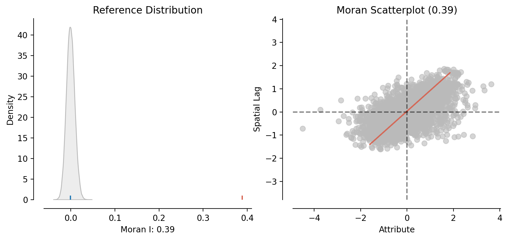

15.1.1 School-Level Achievement Trends

Code

moran_trend = esda.Moran(schools.learning_trend.values, w_school, permutations=99999)

print(f"School-level Moran's I coefficient (trend): {np.round(moran_trend.I,3)}")
print(f"p-value of Moran's I (trend): {np.round(moran_trend.p_sim, 5)}")

School-level Moran's I coefficient (trend): 0.155
p-value of Moran's I (trend): 1e-05

Code

esplt.plot_moran(moran_trend)

(<Figure size 1000x400 with 2 Axes>,
 array([<AxesSubplot:title={'center':'Reference Distribution'}, xlabel='Moran I: 0.16', ylabel='Density'>,
        <AxesSubplot:title={'center':'Moran Scatterplot (0.16)'}, xlabel='Attribute', ylabel='Spatial Lag'>],
       dtype=object))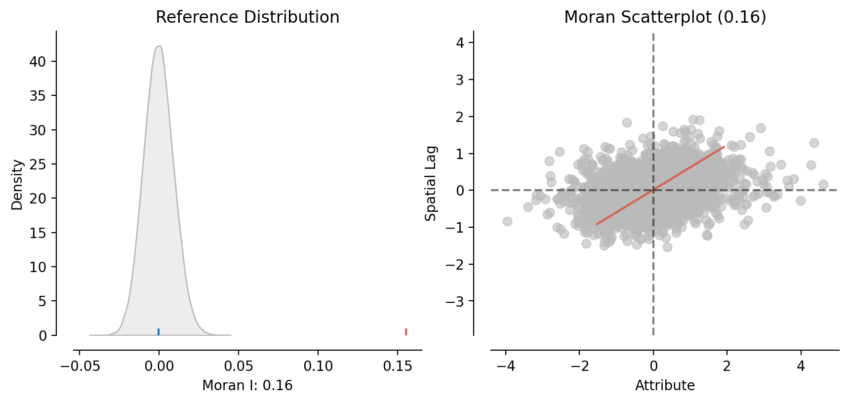

15.2 Exporatory Spatial Data Analysis - “Local” Scale

15.2.1 Average Achievement

Code

lisa_school_avg = esda.Moran_Local(schools.dropna(subset=['avg_score']).avg_score.values, w_school)

esplt.plot_local_autocorrelation(lisa_school_avg, schools, 'avg_score')

(<Figure size 1500x400 with 3 Axes>,
 array([<AxesSubplot:title={'center':'Moran Local Scatterplot'}, xlabel='Attribute', ylabel='Spatial Lag'>,
        <AxesSubplot:>, <AxesSubplot:>], dtype=object))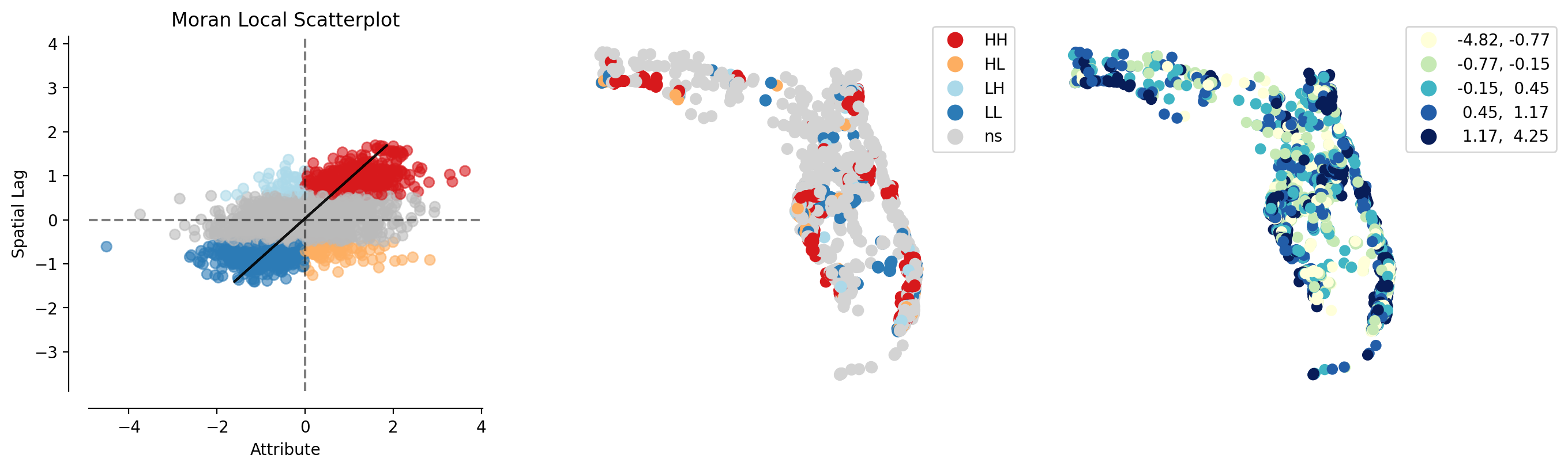

Code

explore_local_moran(
    lisa_school_avg,
    schools,
    "avg_score",
    crit_value=0.01,
    explore_kwargs={
        "marker_kwds": {"radius": 7},
        "tooltip": ["NAME", "avg_score"],
        "tiles": "Stamen Toner Lite",
    },
)

Make this Notebook Trusted to load map: File -> Trust Notebook

15.2.2 Achievement Trend

Repeating the analysis for trends in school-level achievement reveals many of the same patterns, however in this case the value for Moran’s I is much lower.

Code

lisa_school_trend = esda.Moran_Local(schools.dropna(subset=['learning_trend']).learning_trend.values, w_school)

Code

explore_local_moran(
    lisa_school_trend,
    schools,
    "avg_score",
    crit_value=0.01,
    explore_kwargs={
        "marker_kwds": {"radius": 7},
        "tooltip": ["NAME", "avg_score"],
        "tiles": "Stamen Toner Lite",
    },
)

Make this Notebook Trusted to load map: File -> Trust Notebook