8  TX: District-Level Overall Achievement

Code

state = 'tx'

Code

schools = gpd.read_parquet(f"../data/{state}_schools.parquet")
schools = schools.to_crs(schools.estimate_utm_crs())

dists = gpd.read_parquet(f"../data/{state}_dists.parquet")
dists = dists.to_crs(dists.estimate_utm_crs())

schools = schools.dropna(
    subset=["avg_score", "learning_rate", "learning_trend"]
)
dists = dists.dropna(subset=["avg_score", "learning_rate", "learning_trend"])

Note we need to simplify the geometries just a touch to get the map to render

Code

dists['geom_simple'] = dists['geometry'].simplify(500)

Code

dists[["NAME", "avg_score", "geom_simple"]].set_geometry('geom_simple').explore(
    "avg_score",
    scheme="quantiles",
    k=8,
    cmap="PRGn",
    tiles="Stamen Toner Lite",
    marker_kwds={"radius": 7},
    style_kwds={"stroke": False,
               "transparency":0.5},
    tooltip=["NAME", "avg_score"],
)

Make this Notebook Trusted to load map: File -> Trust Notebook

8.1 Exporatory Spatial Data Analysis - “Global” Scale

8.1.1 Average Achievement

Code

w_dist = weights.Rook.from_dataframe(dists)

moran = esda.Moran(dists.avg_score.values, w_dist, permutations=99999)

print(f"District-level Moran's I coefficient: {np.round(moran.I,3)}")

print(f"p-value of Moran's I: {np.round(moran.p_sim, 5)}")

District-level Moran's I coefficient: 0.198
p-value of Moran's I: 1e-05

Code

esplt.plot_moran(moran)

(<Figure size 1000x400 with 2 Axes>,
 array([<AxesSubplot:title={'center':'Reference Distribution'}, xlabel='Moran I: 0.2', ylabel='Density'>,
        <AxesSubplot:title={'center':'Moran Scatterplot (0.2)'}, xlabel='Attribute', ylabel='Spatial Lag'>],
       dtype=object))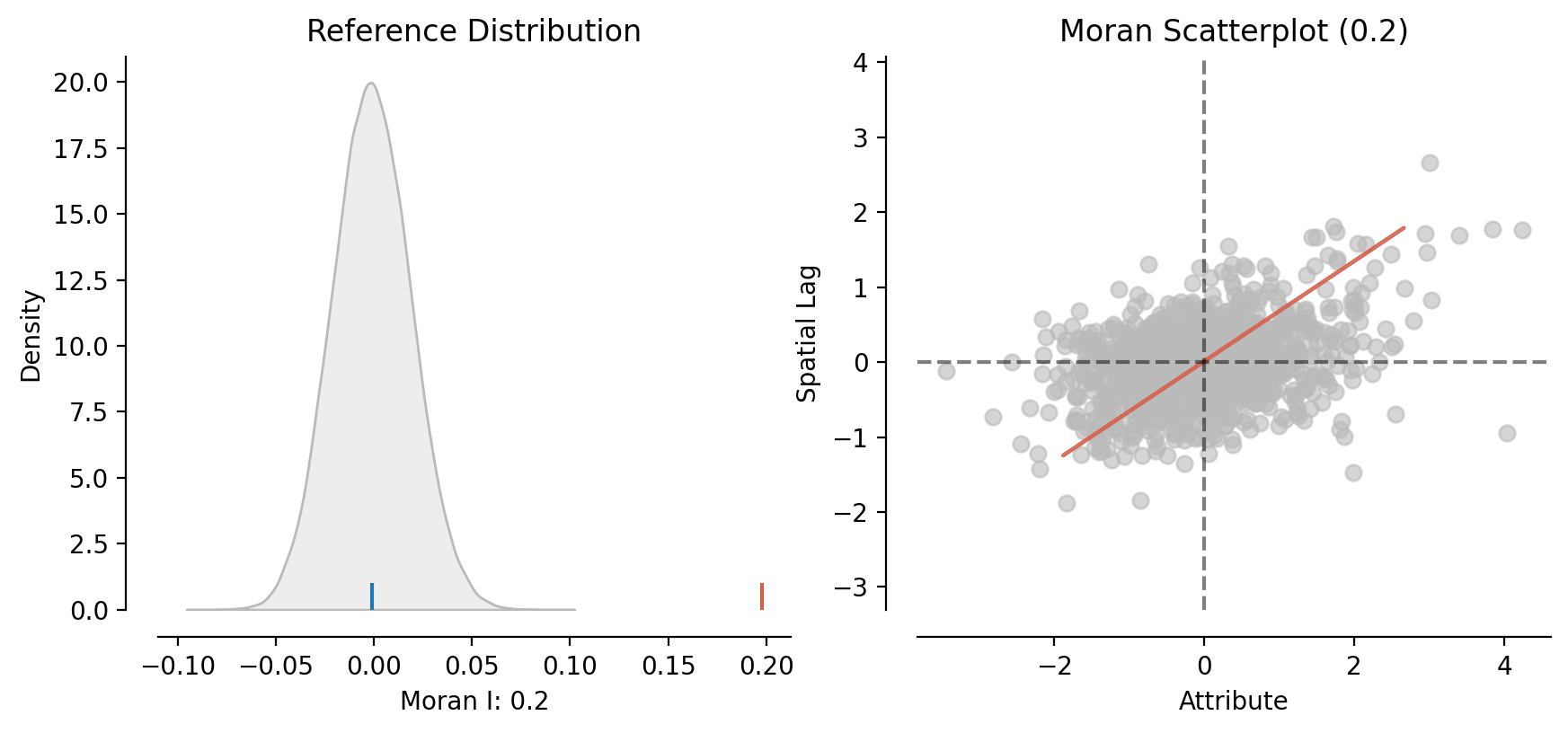

8.1.2 Achievement Trend Over Time

Code

moran = esda.Moran(dists.learning_trend.values, w_dist, permutations=99999)

print(f"District-level Moran's I coefficient (trend): {np.round(moran.I,3)}")

print(f"p-value of Moran's I (trend): {np.round(moran.p_sim, 5)}")

District-level Moran's I coefficient (trend): 0.054
p-value of Moran's I (trend): 0.00368

Code

esplt.plot_moran(moran)

(<Figure size 1000x400 with 2 Axes>,
 array([<AxesSubplot:title={'center':'Reference Distribution'}, xlabel='Moran I: 0.05', ylabel='Density'>,
        <AxesSubplot:title={'center':'Moran Scatterplot (0.05)'}, xlabel='Attribute', ylabel='Spatial Lag'>],
       dtype=object))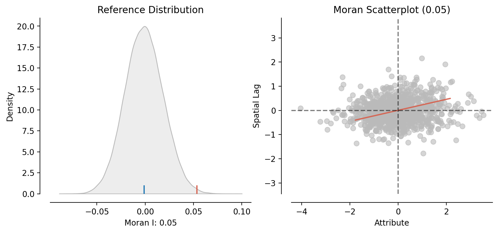

8.2 Exporatory Spatial Data Analysis - “Local” Scale

8.2.1 Average Achievement

In particular, the LISA analysis examines whether each geographic unit (school districts, in this case) has a statistically significant with its neighbors, and if so, it classifies that unit into one of four types:

• High-High: the “HH” label is for high achieving districts surrounded by other high-achieving districts, and these can be viewed as “hotspots”, because the cluster of high-performing districts stands out from those nearby. These observations are colored red.

• High-Low: the “HL” label is for high achieving districts surrounded by low-achieving districts. These observations are sometimes called “diamonds in the rough” because they represent very high values surrounded by very low values. In the contect of educational achievement, these are particularly interesting observations because they represent places that are doing well, despite local trends of underperformance. These observations are colored orange.

• Low-High: the “LH” label is for low-achieving districts surrounded by high-achieving districts. These observations are sometimes called “doughnuts” because they represent a hole surrounded by high values. These are observations that are struggling to keep pace with their high-performing neighbors, and are colored light blue.

• Low-Low: the “LL” label is for low-achieving districts surrounded by low-achieving districts, and these can be viewed as “coldspots” because they reresent a cluster of low-performing districts that standout from the other places nearby.

When an observation is colored gray, it means that it does not have a statistically significant relationship with its neighbors.

Code

lisa_dist_avg = esda.Moran_Local(
    dists.dropna(subset=["avg_score"]).avg_score.values, w_dist
)

explore_local_moran(
    lisa_dist_avg,
    dists.set_geometry('geom_simple'),
    "avg_score",
    explore_kwargs={
        "marker_kwds": {"radius": 7},
        "tooltip": ["NAME", "avg_score"],
        "tiles": "Stamen Toner Lite",
        "style_kwds": {"stroke": False},
    },
)

Make this Notebook Trusted to load map: File -> Trust Notebook

8.2.2 Achievement Trend

Code

lisa_dist_trend = esda.Moran_Local(
    dists.dropna(subset=["learning_trend"]).learning_trend.values, w_dist
)

explore_local_moran(
    lisa_dist_trend,
    dists.set_geometry('geom_simple'),
    "ach_trend",
    explore_kwargs={
        "marker_kwds": {"radius": 7},
        "tooltip": ["NAME", "learning_trend"],
        "tiles": "Stamen Toner Lite",
        "style_kwds": {"stroke": False},
    },
)

Make this Notebook Trusted to load map: File -> Trust Notebook