Bayesian Spatial Flow (Origin–Destination) Models¶
This notebook demonstrates the cross-sectional flow models in bayespecon:
Model |
Description |
|---|---|
|
Three free ρ parameters — destination, origin, network |
|
Constrained ρ_w = −ρ_d·ρ_o; exact eigenvalue log-det |
Both are fully Bayesian implementations of the LeSage–Fischer (2008) SAR flow framework.
Background: The SAR Flow Model¶
Let \(y\) be the \(N\)-vector of observed flows (\(N = n^2\) O-D pairs). The model is
where
capture destination, origin, and network (O-D pair) neighbourhood dependence respectively.
The reduced form is
The design matrix \(X\) follows the LeSage layout with separate destination, origin, and intra-zonal coefficient blocks:
Separable variant¶
SARFlowSeparable imposes \(\rho_w = -\rho_d \rho_o\), which makes the filter matrix factorisable as a Kronecker product:
This enables exact, O(n) log-det evaluation via eigenvalues of the small \(n\times n\) matrix \(W\).
Setup¶
import warnings

import arviz as az
import matplotlib.pyplot as plt
import numpy as np
import pandas as pd

from bayespecon import SARFlow, SARFlowSeparable, flow_design_matrix
from bayespecon.dgp.flows import generate_flow_data, generate_flow_data_separable

warnings.filterwarnings("ignore")
az.style.use("arviz-white")
rng = np.random.default_rng(42)
/home/runner/micromamba/envs/test/lib/python3.14/site-packages/tqdm/auto.py:21: TqdmWarning: IProgress not found. Please update jupyter and ipywidgets. See https://ipywidgets.readthedocs.io/en/stable/user_install.html
  from .autonotebook import tqdm as notebook_tqdm
1 Simulated Data¶
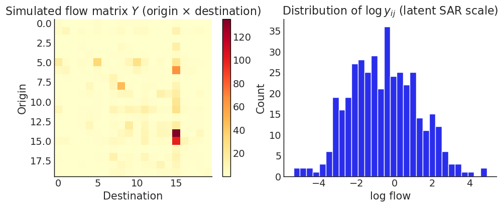
We simulate flow data on \(n = 12\) spatial units, giving \(N = 144\) O-D pairs.
When neither G nor gdf is supplied, generate_flow_data
synthesises a point grid, builds a row-standardised KNN graph
(knn_k=4 by default) and computes the pairwise distance matrix used
for the gravity-style log_distance regressor.
True parameters
Parameter |
Value |
|---|---|
ρ_d |
0.35 |
ρ_o |
0.25 |
ρ_w |
0.10 |
β_d |
[1.0, −0.5] |
β_o |
[0.5, 0.3] |
σ |
1.0 |
γ_dist (log_distance coef.) |
−0.5 (default) |
# True parameters (matching the table above)
RHO_D = 0.35
RHO_O = 0.25
RHO_W = 0.10
BETA_D = [1.0, -0.5]
BETA_O = [0.5, 0.3]
SIGMA = 1.0

# Generate synthetic flow data (auto-builds KNN graph + distance matrix)
data = generate_flow_data(
    n=20,
    rho_d=RHO_D,
    rho_o=RHO_O,
    rho_w=RHO_W,
    beta_d=BETA_D,
    beta_o=BETA_O,
    sigma=SIGMA,
    seed=42,
)

n = 20
N = n * n
G = data["G"]
gdf = data["gdf"]

print(f"Generated {N} O-D flows on {n} spatial units")
print(f"Design matrix: {data['X'].shape}, columns: {data['col_names']}")
print(f"Design: k_d={data['design'].k_d}, k_o={data['design'].k_o}")
Generated 400 O-D flows on 20 spatial units
Design matrix: (400, 9), columns: ['intercept', 'intra_indicator', 'dest_x0', 'dest_x1', 'orig_x0', 'orig_x1', 'intra_x0', 'intra_x1', 'log_distance']
Design: k_d=2, k_o=2
y_obs = data["y_vec"]  # observed (positive) flows
y_vec = np.log(y_obs)  # latent SAR scale (DGP default is lognormal)
X = data["X"]  # (N, p) design matrix (incl. log_distance column)
col_names = data["col_names"]
G = data["G"].transform("r")  # row-standardised KNN graph synthesised by the DGP
gdf = data["gdf"]  # synthetic point GeoDataFrame

print(f"Flow observations: N = {N}  ({n}×{n})")
print(f"Design matrix shape: {X.shape}")
print(f"Column names: {col_names}")
print(f"Last column ({col_names[-1]}) coefficient (gamma_dist) = {data['gamma_dist']}")
print(
    f"\ny (observed) summary:  min={y_obs.min():.2f}  mean={y_obs.mean():.2f}  max={y_obs.max():.2f}"
)
print(
    f"y (log scale) summary:  min={y_vec.min():.2f}  mean={y_vec.mean():.2f}  max={y_vec.max():.2f}"
)
Flow observations: N = 400  (20×20)
Design matrix shape: (400, 9)
Column names: ['intercept', 'intra_indicator', 'dest_x0', 'dest_x1', 'orig_x0', 'orig_x1', 'intra_x0', 'intra_x1', 'log_distance']
Last column (log_distance) coefficient (gamma_dist) = -0.5

y (observed) summary:  min=0.00  mean=2.91  max=134.95
y (log scale) summary:  min=-5.34  mean=-0.56  max=4.90
Note — lognormal default (since v0.2).
generate_flow_datanow returns strictly-positive flows by default, drawn from \(y = \exp(\eta)\) where \(\eta = A^{-1}(X\beta + \varepsilon)\) is the latent SAR-filtered linear predictor (also exposed asdata["eta_vec"]). The Gaussian-likelihood flow models in this notebook (OLSFlow,SARFlow,SARFlowSeparable) operate on the latent scale, so we fit onnp.log(data["y_vec"]). Passdistribution="normal"to recover the legacy Gaussian-on-y behaviour.
# Visualise the flow matrix (observed scale) and the latent log-scale histogram
fig, axes = plt.subplots(1, 2, figsize=(10, 4))

im = axes[0].imshow(y_obs.reshape(n, n), cmap="YlOrRd")
axes[0].set_title("Simulated flow matrix $Y$ (origin × destination)")
axes[0].set_xlabel("Destination")
axes[0].set_ylabel("Origin")
plt.colorbar(im, ax=axes[0])

axes[1].hist(y_vec, bins=30, edgecolor="white")
axes[1].set_title(r"Distribution of $\log y_{ij}$ (latent SAR scale)")
axes[1].set_xlabel("log flow")
axes[1].set_ylabel("Count")

# plt.tight_layout()
plt.show()
2 SARFlow: Three-parameter model¶
SARFlow places a Dirichlet prior on \((ρ_d, ρ_o, ρ_w)\) that enforces positivity and the stability constraint \(\rho_d + \rho_o + \rho_w \leq 1\) exactly, using the stick-breaking transformation for NUTS efficiency.
The log-determinant \(\log|A|\) is evaluated via the Barry–Pace trace-stochastic method, which requires only sparse matrix–vector products.
sar_flow = SARFlow(
    y_vec,
    G,
    X,
    col_names=col_names,
    logdet_method="traces",  # Barry-Pace stochastic trace (default)
    restrict_positive=True,  # Dirichlet stability prior
    miter=20,  # trace polynomial order (increase for better accuracy)
    trace_seed=0,
)

idata_sar = sar_flow.fit(
    draws=1000,
    tune=1000,
    chains=4,
    target_accept=0.9,
    random_seed=42,
    progressbar=True,
)
Initializing NUTS using jitter+adapt_diag...
Multiprocess sampling (4 chains in 2 jobs)
NUTS: [rho_simplex, beta, sigma]
Sampling 4 chains for 1_000 tune and 1_000 draw iterations (4_000 + 4_000 draws total) took 43 seconds.
# Posterior summary for the spatial autoregressive parameters
summary_rho = sar_flow.summary(var_names=["rho_d", "rho_o", "rho_w"])
print("=== SARFlow: spatial autoregressive parameters ===")
print(summary_rho.to_string())

# Compare to true values
print(f"\nTrue values:  rho_d={RHO_D}  rho_o={RHO_O}  rho_w={RHO_W}")
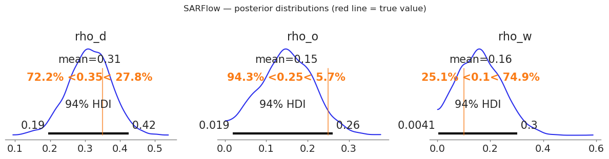
=== SARFlow: spatial autoregressive parameters ===
        mean     sd  hdi_3%  hdi_97%  mcse_mean  mcse_sd  ess_bulk  ess_tail  r_hat
rho_d  0.313  0.062   0.195    0.425      0.001    0.001    2843.0    2762.0    1.0
rho_o  0.149  0.065   0.019    0.260      0.002    0.001    1734.0    1456.0    1.0
rho_w  0.163  0.084   0.004    0.302      0.002    0.001    1923.0    1314.0    1.0

True values:  rho_d=0.35  rho_o=0.25  rho_w=0.1
# Full coefficient summary
summary_beta = sar_flow.summary(var_names=["beta", "sigma"])
print("=== SARFlow: regression coefficients ===")
print(summary_beta.to_string())
=== SARFlow: regression coefficients ===
                        mean     sd  hdi_3%  hdi_97%  mcse_mean  mcse_sd  ess_bulk  ess_tail  r_hat
beta[intercept]        0.310  0.213  -0.094    0.702      0.004    0.004    2294.0    2512.0    1.0
beta[intra_indicator]  0.240  0.323  -0.315    0.889      0.007    0.005    2422.0    2643.0    1.0
beta[dest_x0]          1.113  0.109   0.916    1.323      0.002    0.002    2164.0    2655.0    1.0
beta[dest_x1]         -0.628  0.086  -0.795   -0.474      0.002    0.001    2552.0    2594.0    1.0
beta[orig_x0]          0.501  0.086   0.337    0.657      0.001    0.001    3268.0    2892.0    1.0
beta[orig_x1]          0.332  0.074   0.202    0.476      0.001    0.001    3586.0    2847.0    1.0
beta[intra_x0]         0.052  0.308  -0.494    0.644      0.005    0.005    3639.0    2791.0    1.0
beta[intra_x1]        -0.143  0.329  -0.707    0.525      0.005    0.005    3582.0    2904.0    1.0
beta[log_distance]    -0.877  0.192  -1.228   -0.509      0.004    0.003    2158.0    2704.0    1.0
sigma                  1.001  0.036   0.934    1.068      0.001    0.001    4424.0    2428.0    1.0
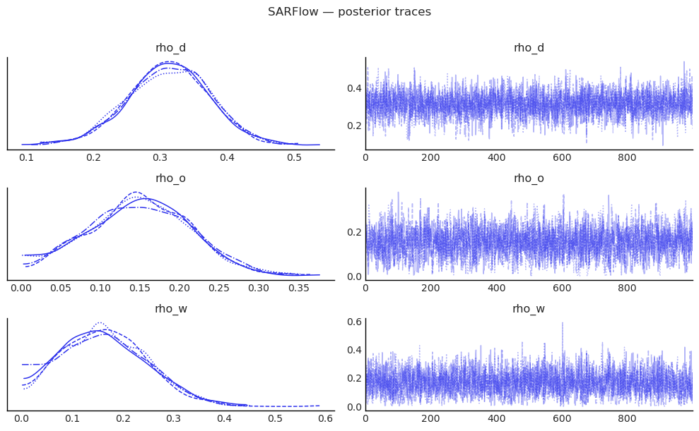
# Trace plots for the three ρ parameters
az.plot_trace(
    idata_sar,
    var_names=["rho_d", "rho_o", "rho_w"],
    figsize=(10, 6),
)
plt.suptitle("SARFlow — posterior traces", y=1.01)
plt.tight_layout()
plt.show()
# Posterior densities with true-value markers
fig, axes = plt.subplots(1, 3, figsize=(12, 3))
params = [("rho_d", RHO_D), ("rho_o", RHO_O), ("rho_w", RHO_W)]

for ax, (param, true_val) in zip(axes, params):
    az.plot_posterior(
        idata_sar,
        var_names=[param],
        ax=ax,
        ref_val=true_val,
        hdi_prob=0.94,
    )
    # ax.set_title(f"${param.replace('_', r'\\_')}$ (true = {true_val})")

plt.suptitle("SARFlow — posterior distributions (red line = true value)", y=1.02)
plt.tight_layout()
plt.show()
3 SARFlowSeparable: Constrained model¶
SARFlowSeparable imposes the constraint \(\rho_w = -\rho_d \rho_o\), yielding:
Exact log-det via eigenvalues of the small \(n \times n\) matrix \(W\) — no Monte Carlo traces needed.
Two free parameters (\(\rho_d\), \(\rho_o\)) instead of three.
Typically faster mixing because the posterior geometry is simpler.
We generate new data that satisfies the constraint (\(\rho_w = -\rho_d\rho_o = -0.12\)) to give the model the best chance at recovery.
# True parameters for the separable model (asymmetric for identifiability)
RHO_D_SEP = 0.40
RHO_O_SEP = 0.30
RHO_W_SEP = -RHO_D_SEP * RHO_O_SEP  # = -0.12 (constraint)

print(
    f"Separable true values:  rho_d={RHO_D_SEP}  rho_o={RHO_O_SEP}"
    f"  rho_w=-rho_d*rho_o={RHO_W_SEP:.4f}"
)

data_sep = generate_flow_data_separable(
    n,
    G,
    rho_d=RHO_D_SEP,
    rho_o=RHO_O_SEP,
    beta_d=BETA_D,
    beta_o=BETA_O,
    sigma=SIGMA,
    seed=7,
)

y_sep = np.log(data_sep["y_vec"])  # latent SAR scale (lognormal default)
X_sep = data_sep["X"]
cn_sep = data_sep["col_names"]

print(
    f"\ny_sep summary:  min={y_sep.min():.2f}  mean={y_sep.mean():.2f}  max={y_sep.max():.2f}"
)
Separable true values:  rho_d=0.4  rho_o=0.3  rho_w=-rho_d*rho_o=-0.1200

y_sep summary:  min=-9.82  mean=-3.48  max=1.70
sep_flow = SARFlowSeparable(
    y_sep,
    G,
    X_sep,
    col_names=cn_sep,
    # logdet_method="eigenvalue" is the default for SARFlowSeparable
    trace_seed=0,
)

idata_sep = sep_flow.fit(
    draws=1000,
    tune=1000,
    chains=4,
    target_accept=0.9,
    random_seed=42,
    progressbar=True,
)
Initializing NUTS using jitter+adapt_diag...
Multiprocess sampling (4 chains in 2 jobs)
NUTS: [rho_d, rho_o, beta, sigma]
Sampling 4 chains for 1_000 tune and 1_000 draw iterations (4_000 + 4_000 draws total) took 15 seconds.
summary_sep = sep_flow.summary(var_names=["rho_d", "rho_o"])
print("=== SARFlowSeparable: spatial autoregressive parameters ===")
print(summary_sep.to_string())
print(
    f"\nTrue values:  rho_d={RHO_D_SEP}  rho_o={RHO_O_SEP}"
    f"  (rho_w = -rho_d*rho_o = {RHO_W_SEP:.4f} is derived)"
)
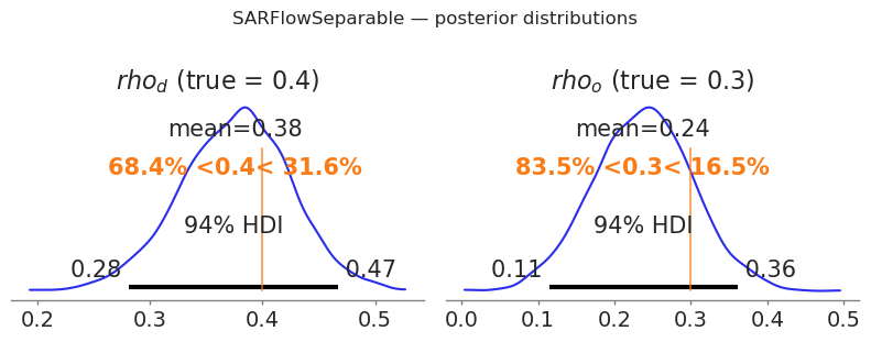
=== SARFlowSeparable: spatial autoregressive parameters ===
        mean     sd  hdi_3%  hdi_97%  mcse_mean  mcse_sd  ess_bulk  ess_tail  r_hat
rho_d  0.376  0.049   0.281    0.467      0.001    0.001    3302.0    2684.0    1.0
rho_o  0.237  0.065   0.114    0.361      0.001    0.001    2582.0    2441.0    1.0

True values:  rho_d=0.4  rho_o=0.3  (rho_w = -rho_d*rho_o = -0.1200 is derived)
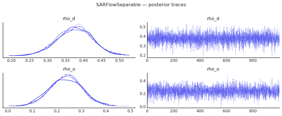
az.plot_trace(
    idata_sep,
    var_names=["rho_d", "rho_o"],
    figsize=(10, 4),
)
plt.suptitle("SARFlowSeparable — posterior traces", y=1.01)
plt.tight_layout()
plt.show()
fig, axes = plt.subplots(1, 2, figsize=(8, 3))
for ax, (param, true_val) in zip(axes, [("rho_d", RHO_D_SEP), ("rho_o", RHO_O_SEP)]):
    az.plot_posterior(
        idata_sep, var_names=[param], ax=ax, ref_val=true_val, hdi_prob=0.94
    )
    ax.set_title(f"${param.replace('_', r'_')}$ (true = {true_val})")

plt.suptitle("SARFlowSeparable — posterior distributions", y=1.02)
plt.tight_layout()
plt.show()
4 Design Matrix Details¶
The flow_design_matrix helper builds the standard LeSage O-D design matrix with destination, origin, and intra-zonal coefficient blocks. Each column of the regional attribute matrix \(X\) (shape \(n \times k\)) produces three columns in the full design matrix: one for destination effects, one for origin effects, and one for intra-zonal effects.
Column group |
Construction |
Interpretation |
|---|---|---|
intercept |
\(\mathbf{1}_N\) |
global mean flow |
intra_indicator |
\(\text{vec}(I_n)\) |
intra-zonal dummy |
dest_* |
\(\iota_n \otimes X\) |
destination characteristics |
orig_* |
\(X \otimes \iota_n\) |
origin characteristics |
intra_* |
\(\text{diag}(I_n) \cdot (I_n \otimes X)\) |
intra-zonal attr. |
log_distance |
\(\log(1 + d_{ij})\) |
gravity distance decay |
By default the DGP appends a log_distance column built from
\(\log(1 + d_{ij})\) and assigns it the coefficient gamma_dist=-0.5
(set gamma_dist=0.0 to neutralise the effect). When you build a
design matrix by hand via flow_design_matrix, pass dist=...
together with log_distance=True to include the same column.
You can also pass a pre-built pd.DataFrame directly as X — column names are inferred automatically.
# Build a design matrix from scratch using regional attributes
X_regional = rng.standard_normal((n, 2))  # n × k attribute matrix
dm = flow_design_matrix(X_regional, col_names=["income", "pop"])

print(f"Regional attribute matrix: {X_regional.shape}  (n × k)")
print(f"Full O-D design matrix:    {dm.combined.shape}  (N × p)")
print(f"\nColumn names:\n  {dm.feature_names}")

pd.DataFrame(dm.combined[:6], columns=dm.feature_names).round(3)
Regional attribute matrix: (20, 2)  (n × k)
Full O-D design matrix:    (400, 8)  (N × p)

Column names:
  ['intercept', 'intra_indicator', 'dest_income', 'dest_pop', 'orig_income', 'orig_pop', 'intra_income', 'intra_pop']
| intercept | intra_indicator | dest_income | dest_pop | orig_income | orig_pop | intra_income | intra_pop | |
|---|---|---|---|---|---|---|---|---|
| 0 | 1.0 | 1.0 | 0.305 | -1.040 | 0.305 | -1.04 | 0.305 | -1.04 |
| 1 | 1.0 | 0.0 | 0.750 | 0.941 | 0.305 | -1.04 | 0.000 | 0.00 |
| 2 | 1.0 | 0.0 | -1.951 | -1.302 | 0.305 | -1.04 | -0.000 | -0.00 |
| 3 | 1.0 | 0.0 | 0.128 | -0.316 | 0.305 | -1.04 | 0.000 | -0.00 |
| 4 | 1.0 | 0.0 | -0.017 | -0.853 | 0.305 | -1.04 | -0.000 | -0.00 |
| 5 | 1.0 | 0.0 | 0.879 | 0.778 | 0.305 | -1.04 | 0.000 | 0.00 |
5 Spatial Effects¶
The flow SAR model has a rich effects decomposition due to
:cite:t:thomas-agnan2014SpatialEconometric (chapter 83, §83.5). For each
regional predictor \(p\), a unit shock to \(X_d^{(p)}\) (destination side) and a
unit shock to \(X_o^{(p)}\) (origin side) propagate through the spatial filter
\(A = I_N - \rho_d W_d - \rho_o W_o - \rho_w W_w\) to produce five scalar
summaries (averaged across the \(n\) perturbed regions):
Effect |
Symbol |
Cells aggregated |
|---|---|---|
Origin |
OE |
flows whose origin matches the perturbed region |
Destination |
DE |
flows whose destination matches the perturbed region |
Intra |
IE |
the diagonal \((j, j)\) flow of the perturbed region |
Network |
NE |
all remaining flows |
Total |
TE |
OE + DE + IE + NE |
The high-level wrapper model.spatial_effects() returns a tidy DataFrame.
Three modes are supported:
mode="auto"(default) — combined (sum of dest+orig) when \(X_o = X_d\), otherwise separate.mode="combined"— always sum dest and orig contributions.mode="separate"— always report both sides (Thomas-Agnan §83.5.2).
When intra_* columns are present the destination shock also carries
\(\beta_\text{intra}\) at the diagonal cell, since the design matrix sets
X_intra = intra_indicator · X_dest.
# Combined effects (default for symmetric Xo == Xd designs).
effects_df = sar_flow.spatial_effects(mode="combined")
effects_df.round(4)
| mean | ci_lower | ci_upper | bayes_pvalue | |||
|---|---|---|---|---|---|---|
| predictor | side | effect | ||||
| x0 | combined | origin | 0.8173 | 0.5985 | 1.0541 | 0.0000 |
| x1 | combined | origin | 0.4370 | 0.2379 | 0.6422 | 0.0000 |
| x0 | combined | destination | 1.3987 | 1.2107 | 1.6189 | 0.0000 |
| x1 | combined | destination | -0.7532 | -0.9258 | -0.5728 | 0.0000 |
| x0 | combined | intra | 0.1133 | 0.0830 | 0.1454 | 0.0000 |
| x1 | combined | intra | -0.0224 | -0.0544 | 0.0102 | 0.1865 |
| x0 | combined | network | 2.1345 | 1.0830 | 3.9727 | 0.0000 |
| x1 | combined | network | -0.5053 | -1.0672 | -0.1235 | 0.0060 |
| x0 | combined | total | 4.4639 | 3.1425 | 6.6396 | 0.0000 |
| x1 | combined | total | -0.8439 | -1.6447 | -0.2163 | 0.0070 |
# Small sampler settings used for the demo fits below.
SAMPLE_KWARGS_DEMO = dict(
    draws=200, tune=200, chains=2, random_seed=0, progressbar=False
)
5.1 Asymmetric origin / destination attributes¶
When destination and origin attribute matrices have different numbers of columns (k_d ≠ k_o), pass beta_d and beta_o with different lengths to generate_flow_data. The design matrix layout becomes:
intercept | intra_indicator | dest_*(k_d) | orig_*(k_o) | intra_*(k_d) | dist
The model auto-detects k_d and k_o from column name prefixes (dest_* vs orig_*). spatial_effects() reports destination and origin effects separately when k_d ≠ k_o, since the predictors are different variables.
from bayespecon.dgp.flows import generate_flow_data

# Asymmetric: 2 destination attributes, 1 origin attribute
data_asym = generate_flow_data(
    n=5,
    rho_d=0.2,
    rho_o=0.15,
    rho_w=0.05,
    beta_d=[1.0, -0.5],  # k_d = 2
    beta_o=[0.5],  # k_o = 1
    sigma=0.5,
    seed=11,
)
G_asym = data_asym["G"]
print(f"k_d={data_asym['design'].k_d}, k_o={data_asym['design'].k_o}")
print(f"Columns: {data_asym['col_names']}")

model_asym = SARFlow(
    np.log(data_asym["y_vec"]),
    G_asym,
    data_asym["X"],
    col_names=data_asym["col_names"],
)
print("symmetric_xo_xd =", model_asym._symmetric_xo_xd)
model_asym.fit(**SAMPLE_KWARGS_DEMO)
model_asym.spatial_effects().round(4)  # auto -> separate
k_d=2, k_o=1
Columns: ['intercept', 'intra_indicator', 'dest_x0', 'dest_x1', 'orig_y0', 'intra_x0', 'intra_x1', 'log_distance']
symmetric_xo_xd = False
Initializing NUTS using jitter+adapt_diag...
Multiprocess sampling (2 chains in 2 jobs)
NUTS: [rho_simplex, beta, sigma]
Sampling 2 chains for 200 tune and 200 draw iterations (400 + 400 draws total) took 20 seconds.
We recommend running at least 4 chains for robust computation of convergence diagnostics
The rhat statistic is larger than 1.01 for some parameters. This indicates problems during sampling. See https://arxiv.org/abs/1903.08008 for details
The effective sample size per chain is smaller than 100 for some parameters.  A higher number is needed for reliable rhat and ess computation. See https://arxiv.org/abs/1903.08008 for details
| mean | ci_lower | ci_upper | bayes_pvalue | |||
|---|---|---|---|---|---|---|
| predictor | side | effect | ||||
| x0 | dest | origin | 0.6935 | 0.0472 | 3.5961 | 0.000 |
| x1 | dest | origin | -0.3707 | -1.9262 | -0.0185 | 0.005 |
| x0 | dest | destination | 1.4260 | 0.5755 | 4.2631 | 0.000 |
| x1 | dest | destination | -0.8661 | -2.4445 | -0.3966 | 0.000 |
| x0 | dest | intra | 0.3860 | 0.1102 | 1.2336 | 0.010 |
| x1 | dest | intra | -0.1657 | -0.5729 | -0.0104 | 0.020 |
| x0 | dest | network | 2.7091 | 0.1900 | 13.8080 | 0.000 |
| x1 | dest | network | -1.5873 | -8.0320 | -0.1167 | 0.000 |
| x0 | dest | total | 5.2146 | 1.1387 | 22.9015 | 0.000 |
| x1 | dest | total | -2.9898 | -12.9390 | -0.5968 | 0.000 |
| y0 | orig | origin | 0.8246 | 0.2467 | 2.3855 | 0.005 |
| destination | 0.2712 | 0.0112 | 1.9070 | 0.005 | ||
| intra | 0.2062 | 0.0617 | 0.5964 | 0.005 | ||
| network | 1.0850 | 0.0449 | 7.6279 | 0.005 | ||
| total | 2.3870 | 0.4227 | 12.5237 | 0.005 |
# You can also build asymmetric designs directly with flow_design_matrix_asymmetric
from bayespecon.graph import flow_design_matrix_asymmetric

rng_asym = np.random.default_rng(7)
n_demo = 5
Xd = rng_asym.standard_normal((n_demo, 2))  # 2 destination variables
Xo = rng_asym.standard_normal((n_demo, 1))  # 1 origin variable

dm = flow_design_matrix_asymmetric(Xd, Xo)
print(f"Design shape: {dm.combined.shape}")
print(f"k_d={dm.k_d}, k_o={dm.k_o}")
print(f"Feature names: {dm.feature_names}")
Design shape: (25, 7)
k_d=2, k_o=1
Feature names: ['intercept', 'intra_indicator', 'dest_x0', 'dest_x1', 'orig_y0', 'intra_x0', 'intra_x1']
5.2 Non-spatial OLS gravity baseline (OLSFlow)¶
OLSFlow is the conventional log-linear gravity model
(Thomas-Agnan & LeSage 2014, eq. 83.2): no spatial-lag terms, just
\(y = X \beta + \varepsilon\) with iid Gaussian errors. It uses the
same spatial_effects() API and reproduces the closed-form
expressions in Table 83.1 (with \(A = I_N\)):
from bayespecon import OLSFlow

ols_flow = OLSFlow(y_vec, G, X, col_names=col_names)
ols_flow.fit(**SAMPLE_KWARGS_DEMO)
ols_flow.spatial_effects(mode="combined").round(4)
Initializing NUTS using jitter+adapt_diag...
Multiprocess sampling (2 chains in 2 jobs)
NUTS: [beta, sigma]
Sampling 2 chains for 200 tune and 200 draw iterations (400 + 400 draws total) took 5 seconds.
We recommend running at least 4 chains for robust computation of convergence diagnostics
The rhat statistic is larger than 1.01 for some parameters. This indicates problems during sampling. See https://arxiv.org/abs/1903.08008 for details
| mean | ci_lower | ci_upper | bayes_pvalue | |||
|---|---|---|---|---|---|---|
| predictor | side | effect | ||||
| x0 | combined | origin | 0.6549 | 0.5017 | 0.8178 | 0.000 |
| x1 | combined | origin | 0.4752 | 0.3291 | 0.6382 | 0.000 |
| x0 | combined | destination | 1.2144 | 1.0932 | 1.3369 | 0.000 |
| x1 | combined | destination | -0.6934 | -0.8356 | -0.5313 | 0.000 |
| x0 | combined | intra | 0.0980 | 0.0669 | 0.1288 | 0.000 |
| x1 | combined | intra | -0.0135 | -0.0479 | 0.0240 | 0.425 |
| x0 | combined | network | 0.0000 | 0.0000 | 0.0000 | 0.000 |
| x1 | combined | network | 0.0000 | 0.0000 | 0.0000 | 0.000 |
| x0 | combined | total | 1.9673 | 1.7546 | 2.1693 | 0.000 |
| x1 | combined | total | -0.2317 | -0.4353 | -0.0178 | 0.040 |
6 MCMC Diagnostics¶
Good practice after any Bayesian fit: check \(\hat{R}\) (should be \(< 1.01\)) and effective sample size (ESS > 400 per chain).
for label, idata in [("SARFlow", idata_sar), ("SARFlowSeparable", idata_sep)]:
    diag = az.summary(idata, var_names=["rho_d", "rho_o"], stat_focus="mean")
    rhat_ok = (diag["r_hat"] < 1.01).all()
    ess_ok = (diag["ess_bulk"] > 400).all()
    print(f"{label:25s}  r_hat<1.01: {rhat_ok}   ess_bulk>400: {ess_ok}")
    print(diag[["mean", "sd", "hdi_3%", "hdi_97%", "ess_bulk", "r_hat"]].to_string())
    print()
SARFlow                    r_hat<1.01: True   ess_bulk>400: True
        mean     sd  hdi_3%  hdi_97%  ess_bulk  r_hat
rho_d  0.313  0.062   0.195    0.425    2843.0    1.0
rho_o  0.149  0.065   0.019    0.260    1734.0    1.0

SARFlowSeparable           r_hat<1.01: True   ess_bulk>400: True
        mean     sd  hdi_3%  hdi_97%  ess_bulk  r_hat
rho_d  0.376  0.049   0.281    0.467    3302.0    1.0
rho_o  0.237  0.065   0.114    0.361    2582.0    1.0
Spatial-parameter adequacy¶
Flow models have three spatial scalars (\(\rho_d\), \(\rho_o\), \(\rho_w\)),
and each is prone to the slow-mixing behaviour discussed in Wolf,
Anselin & Arribas-Bel (2018) [Wolf et al., 2018].
The spatial_mcmc_diagnostic helper auto-detects all three and reports
ESS, sampler yield, \(\hat{R}\), and HPDI stability.
from bayespecon import spatial_mcmc_diagnostic

spatial_mcmc_diagnostic(sar_flow, emit_warnings=False).to_frame()
| ess_bulk | ess_tail | r_hat | mcse_mean | yield_pct | hpdi_drift_pct | adequate | |
|---|---|---|---|---|---|---|---|
| parameter | |||||||
| rho_d | 2843.361415 | 2762.213487 | 1.000223 | 0.001161 | 71.084035 | 3.094096 | True |
| rho_o | 1733.874492 | 1456.398644 | 1.000084 | 0.001517 | 43.346862 | 3.669676 | True |
| rho_w | 1922.704039 | 1314.145311 | 1.000431 | 0.001806 | 48.067601 | 2.037551 | True |
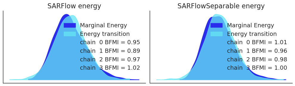
# Energy plot — checks that HMC is exploring the posterior efficiently
fig, axes = plt.subplots(1, 2, figsize=(10, 3))
az.plot_energy(idata_sar, ax=axes[0])
axes[0].set_title("SARFlow energy")
az.plot_energy(idata_sep, ax=axes[1])
axes[1].set_title("SARFlowSeparable energy")
plt.tight_layout()
plt.show()
7 Model Comparison¶
The WAIC / LOO-CV scores can be used to compare SARFlow and SARFlowSeparable when both are estimated on the same data. A lower ELPD (expected log pointwise predictive density) indicates a worse-fitting model.
Note: here we fit
SARFlowto the separable data to make the comparison meaningful — the separable model is nested in the unrestricted one.
# Fit unrestricted SARFlow on the same separable data for a fair comparison
sar_flow_on_sep = SARFlow(
    y_sep,
    G,
    X_sep,
    col_names=cn_sep,
    logdet_method="traces",
    miter=20,
    trace_seed=0,
)
idata_sar_on_sep = sar_flow_on_sep.fit(
    draws=1000,
    tune=1000,
    chains=4,
    target_accept=0.9,
    random_seed=42,
    progressbar=True,
)
Initializing NUTS using jitter+adapt_diag...
Multiprocess sampling (4 chains in 2 jobs)
NUTS: [rho_simplex, beta, sigma]
Sampling 4 chains for 1_000 tune and 1_000 draw iterations (4_000 + 4_000 draws total) took 92 seconds.
# LOO-CV comparison (requires log-likelihood in idata; falls back to WAIC if unavailable)
try:
    loo_sar = az.loo(idata_sar_on_sep)
    loo_sep = az.loo(idata_sep)
    comparison = az.compare(
        {"SARFlow (3 ρ)": idata_sar_on_sep, "SARFlowSeparable": idata_sep}
    )
    print("LOO-CV model comparison:")
    print(
        comparison[
            ["elpd_loo", "p_loo", "elpd_diff", "weight", "se", "warning"]
        ].to_string()
    )
except Exception as e:
    print(f"LOO not available (log-likelihood not stored): {e}")
    print("Tip: pass compute_log_likelihood=True to fit() to enable LOO/WAIC.")
LOO-CV model comparison:
                    elpd_loo      p_loo  elpd_diff    weight         se  warning
SARFlow (3 ρ)    -561.708235  10.847153   0.000000  0.563627  14.016578    False
SARFlowSeparable -561.842865  10.618886   0.134629  0.436373  13.902860    False
8 Prior Sensitivity and Stability Constraint¶
By default SARFlow uses a Dirichlet prior that forces \(\rho_d, \rho_o, \rho_w \geq 0\) and \(\rho_d + \rho_o + \rho_w \leq 1\). Setting restrict_positive=False allows negative spillovers via independent Uniform(-1, 1) priors plus a differentiable stability wall potential.
Use restrict_positive=False when competitive effects (e.g. negative network parameter) are theoretically expected.
# Fit with restrict_positive=False to allow negative rho values
sar_flow_neg = SARFlow(
    y_vec,
    G,
    X,
    col_names=col_names,
    logdet_method="traces",
    restrict_positive=False,  # Uniform(-1,1) priors + stability potential
    miter=20,
    trace_seed=0,
)
idata_neg = sar_flow_neg.fit(
    draws=800,
    tune=1000,
    chains=4,
    target_accept=0.95,
    random_seed=42,
    progressbar=True,
)

summary_neg = sar_flow_neg.summary()
print("=== SARFlow (restrict_positive=False) ===")
print(summary_neg[["mean", "sd", "hdi_3%", "hdi_97%", "r_hat"]].to_string())
Initializing NUTS using jitter+adapt_diag...
Multiprocess sampling (4 chains in 2 jobs)
NUTS: [rho_d, rho_o, rho_w, beta, sigma]
Sampling 4 chains for 1_000 tune and 800 draw iterations (4_000 + 3_200 draws total) took 39 seconds.
=== SARFlow (restrict_positive=False) ===
                        mean     sd  hdi_3%  hdi_97%  r_hat
rho_d                  0.317  0.062   0.203    0.439    1.0
rho_o                  0.149  0.069   0.021    0.279    1.0
rho_w                  0.156  0.096  -0.024    0.337    1.0
beta[intercept]        0.310  0.212  -0.122    0.687    1.0
beta[intra_indicator]  0.245  0.319  -0.305    0.877    1.0
beta[dest_x0]          1.113  0.113   0.895    1.318    1.0
beta[dest_x1]         -0.627  0.089  -0.795   -0.458    1.0
beta[orig_x0]          0.498  0.086   0.346    0.667    1.0
beta[orig_x1]          0.330  0.074   0.192    0.465    1.0
beta[intra_x0]         0.051  0.301  -0.485    0.637    1.0
beta[intra_x1]        -0.147  0.327  -0.745    0.465    1.0
beta[log_distance]    -0.878  0.192  -1.264   -0.538    1.0
sigma                  1.000  0.036   0.930    1.063    1.0
10 Bayesian LM Diagnostics¶
Once a baseline gravity model has been fit, the Bayesian Lagrange-multiplier
(LM) tests in bayespecon.diagnostics indicate which spatial-lag directions
(destination, origin, network) are worth adding — and which intra-block
columns deserve their own coefficients. They are the OD-flow analogues of the
classic Anselin/Koley–Bera LM family, ported to the posterior-predictive
score formulation of Doğan, Taşpınar & Bera (2021).
For each posterior draw \(g\) from a fitted null model with residuals \(e_g = y - X\beta_g\), the score for direction \(i \in \{d, o, w\}\) is
and the information matrix uses the cached Kronecker-trace block
\(T_{\text{flow}}\) (computed in \(\mathcal{O}(\mathrm{nnz})\) from
flow_trace_blocks(W)):
The marginal statistic is \(LM_g = (s_g^{(i)})^2 / J_{ii}\) (\(\chi^2_1\)); the joint statistic is \(g_g^\top J^{-1} g_g\) (\(\chi^2_3\)). The Bayesian \(p\)-value reports \(1 - F_{\chi^2_{\text{df}}}(\overline{LM})\).
10.1 Robust (Neyman-orthogonal) tests¶
The marginal LM tests assume the other two ρ parameters are zero under the null. When that assumption is in doubt, evaluate the score and information at the alternative SARFlow posterior and apply the Neyman-orthogonal adjustment
where \(\nu\) indexes the two nuisance directions. The result is robust to local misspecification of the nuisance ρ’s (Doğan et al. 2021, Proposition 3).
from bayespecon.diagnostics.lmtests import (
    bayesian_robust_lm_flow_dest_test,
    bayesian_robust_lm_flow_network_test,
    bayesian_robust_lm_flow_orig_test,
)

robust_tests = {
    "rho_d | (rho_o, rho_w)": bayesian_robust_lm_flow_dest_test(sar_flow),
    "rho_o | (rho_d, rho_w)": bayesian_robust_lm_flow_orig_test(sar_flow),
    "rho_w | (rho_d, rho_o)": bayesian_robust_lm_flow_network_test(sar_flow),
}

pd.DataFrame(
    [(k, r.mean, r.bayes_pvalue) for k, r in robust_tests.items()],
    columns=["test", "LM* mean", "Bayes p"],
).round(4)
| test | LM* mean | Bayes p | |
|---|---|---|---|
| 0 | rho_d | (rho_o, rho_w) | 1.7096 | 0.1910 |
| 1 | rho_o | (rho_d, rho_w) | 0.7872 | 0.3749 |
| 2 | rho_w | (rho_d, rho_o) | 0.8297 | 0.3623 |
10.2 Panel analogues¶
For a fitted OLSFlowPanel,
the same tests are available with the bayesian_panel_lm_flow_* prefix.
Scores accumulate over the demeaned panel stack of length \(n^2 \cdot T\)
and the information matrix scales the trace block by \(T\) to reflect i.i.d.
within-period contributions under \(H_0\):
from bayespecon import (
    bayesian_panel_lm_flow_dest_test,
    bayesian_panel_lm_flow_orig_test,
    bayesian_panel_lm_flow_network_test,
    bayesian_panel_lm_flow_joint_test,
    bayesian_panel_lm_flow_intra_test,
)
11 Quick Reference¶
from bayespecon import OLSFlow, SARFlow, SARFlowSeparable
from bayespecon import flow_design_matrix
from bayespecon.dgp.flows import generate_flow_data, generate_flow_data_separable

# Build design matrix from regional attributes
dm = flow_design_matrix(X_regional, col_names=["income", "pop"])

# --- SARFlow (three free ρ parameters) ---
model = SARFlow(
    y, G, dm.combined,
    col_names=dm.feature_names,
    logdet_method="traces",      # Barry-Pace stochastic traces (default)
    restrict_positive=True,      # Dirichlet stability prior
)
idata = model.fit(draws=2000, tune=1000, chains=4, random_seed=0)
model.summary(var_names=["rho_d", "rho_o", "rho_w"])

# --- SARFlowSeparable (ρ_w = -ρ_d·ρ_o, exact log-det) ---
sep_model = SARFlowSeparable(
    y, G, dm.combined,
    col_names=dm.feature_names,
    # logdet_method="eigenvalue" is the default
)
idata_sep = sep_model.fit(draws=2000, tune=1000, chains=4, random_seed=0)

# --- OLSFlow (non-spatial gravity baseline) ---
ols = OLSFlow(y, G, dm.combined, col_names=dm.feature_names)
idata_ols = ols.fit(draws=2000, tune=1000, chains=4, random_seed=0)
ols.spatial_effects(mode="combined")  # closed-form Table 83.1

# --- OLSFlow (non-spatial gravity baseline) ---
ols = OLSFlow(y, G, dm.combined, col_names=dm.feature_names)
idata_ols = ols.fit(draws=2000, tune=1000, chains=4, random_seed=0)
ols.spatial_effects(mode="combined")  # closed-form Table 83.1
Key parameters¶
Parameter |
Default |
Description |
|---|---|---|
|
|
|
|
|
Dirichlet prior; set |
|
30 |
Trace polynomial order (higher = more accurate, slower precomputation) |
|
50 |
Monte Carlo probes for trace estimation |
Model choice guide¶
Data characteristic |
Recommended model |
|---|---|
No prior on sign of spatial effects |
|
Positive spillovers expected |
|
Separability plausible, fast inference needed |
|
Count/non-negative flows |
|