SAR Sampling Backend Profiling
Note: To run this notebook you must have optional backends installed, e.g. conda install numpyro blackjax nutpie
This notebook profiles a fixed SAR model across PyMC sampling backends on a regular polygon grid benchmark.
The comparison keeps the SAR specification and log-determinant method fixed and varies the sampling backend only.
The workflow uses the public bayespecon API end to end:
bayespecon.dgp.simulate_sar(..., create_gdf=True)generates synthetic data and returns a GeoDataFrameA libpysal contiguity graph is built from the returned GeoDataFrame
bayespecon.SAR(...)constructs the modelSAR.fit(...)runs each backend
Dataset setup:
n_side × n_sideregular polygon grid (obs = n_side²) generated bybayespecon.dgpone intercept and two continuous regressors
a SAR data-generating process simulated from
bayespecon.dgp
Backends compared:
c: PyMC NUTS with the default C-backedFAST_RUNcompilation modenumba: PyMC NUTS withNUMBAcompilation modenumpyro: JAX-backed NUTS via NumPyroblackjax: JAX-backed NUTS via BlackJAXnutpie: Rust + Numba NUTS via nutpie
The notebook records runtime, posterior means, and divergence counts. Backends that are unavailable in the current environment are skipped automatically.
import importlib.util
import time

import matplotlib.pyplot as plt
import numpy as np
import pandas as pd
from libpysal import graph

from bayespecon import SAR, dgp
PROFILE_CFG = {
    "n_side": 16,  # grid side; obs = n_side² = 256
    "draws": 250,
    "tune": 250,
    "chains": 4,
    "cores": 2,
    "seed": 2026,
    "logdet_method": "eigenvalue",
}

BACKENDS = {
    "c": {
        "nuts_sampler": "pymc",
        "compile_kwargs": {"mode": "FAST_RUN"},
        "requires": [],
    },
    "numba": {
        "nuts_sampler": "pymc",
        "compile_kwargs": {"mode": "NUMBA"},
        "requires": ["numba"],
    },
    "numpyro": {
        "nuts_sampler": "numpyro",
        "compile_kwargs": None,
        "requires": ["numpyro"],
    },
    "blackjax": {
        "nuts_sampler": "blackjax",
        "compile_kwargs": None,
        "requires": ["blackjax"],
    },
    "nutpie": {
        "nuts_sampler": "nutpie",
        "compile_kwargs": None,
        "requires": ["nutpie"],
    },
}

TRUE_BETA = np.array([1.0, 0.8, -0.5], dtype=np.float64)
TRUE_RHO = 0.35
TRUE_SIGMA = 0.7
def backend_available(requirements: list[str]) -> bool:
    return all(importlib.util.find_spec(name) is not None for name in requirements)


def simulate_sar_data(seed: int, n_side: int = 16):
    """Simulate SAR data on an n_side × n_side polygon grid.

    Calls ``dgp.simulate_sar`` with ``create_gdf=True``, then builds a
    libpysal contiguity graph from the returned GeoDataFrame.
    """
    rng = np.random.default_rng(seed)
    gdf = dgp.simulate_sar(
        n=n_side,
        rho=TRUE_RHO,
        beta=TRUE_BETA,
        sigma=TRUE_SIGMA,
        rng=rng,
        create_gdf=True,
    )
    W_graph = graph.Graph.build_contiguity(gdf, rook=True).transform("r")
    y = gdf["y"].to_numpy()
    X_cols = [c for c in gdf.columns if c.startswith("X_")]
    X = gdf[X_cols].to_numpy()
    return gdf, y, X, W_graph


def fit_backend(backend_name: str, y: np.ndarray, X: np.ndarray, W) -> dict:
    cfg = BACKENDS[backend_name]
    if not backend_available(cfg["requires"]):
        return {
            "backend": backend_name,
            "available": False,
            "total_time_s": np.nan,
            "rho_hat": np.nan,
            "beta_0_hat": np.nan,
            "beta_1_hat": np.nan,
            "beta_2_hat": np.nan,
            "divergences": np.nan,
            "error": "missing optional dependency",
        }

    t0 = time.perf_counter()
    try:
        model = SAR(
            y=y,
            X=X,
            W=W,
            logdet_method=PROFILE_CFG["logdet_method"],
        )
        idata = model.fit(
            draws=PROFILE_CFG["draws"],
            tune=PROFILE_CFG["tune"],
            chains=PROFILE_CFG["chains"],
            cores=PROFILE_CFG["cores"],
            random_seed=PROFILE_CFG["seed"],
            progressbar=False,
            compute_convergence_checks=False,
            nuts_sampler=cfg["nuts_sampler"],
            compile_kwargs=cfg["compile_kwargs"],
        )
        elapsed_s = time.perf_counter() - t0

        beta_hat = idata.posterior["beta"].mean(("chain", "draw")).to_numpy()
        rho_hat = float(idata.posterior["rho"].mean(("chain", "draw")).to_numpy())
        divergences = int(idata.sample_stats["diverging"].sum().to_numpy())

        return {
            "backend": backend_name,
            "available": True,
            "total_time_s": elapsed_s,
            "rho_hat": rho_hat,
            "beta_0_hat": float(beta_hat[0]),
            "beta_1_hat": float(beta_hat[1]),
            "beta_2_hat": float(beta_hat[2]),
            "divergences": divergences,
            "error": "",
        }
    except Exception as exc:
        return {
            "backend": backend_name,
            "available": True,
            "total_time_s": np.nan,
            "rho_hat": np.nan,
            "beta_0_hat": np.nan,
            "beta_1_hat": np.nan,
            "beta_2_hat": np.nan,
            "divergences": np.nan,
            "error": f"{type(exc).__name__}: {exc}",
        }
gdf_subset, y, X, W = simulate_sar_data(
seed=PROFILE_CFG["seed"], n_side=PROFILE_CFG["n_side"]
)
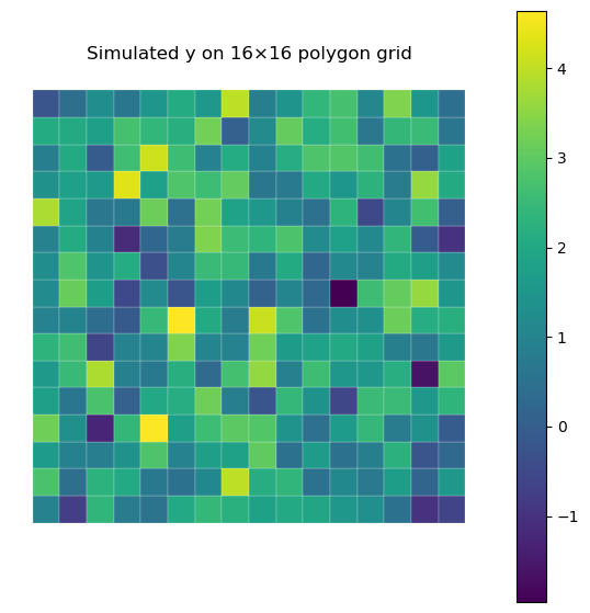
fig, ax = plt.subplots(1, 1, figsize=(7, 7))
gdf_subset.plot(
column="y", cmap="viridis", legend=True, linewidth=0.15, edgecolor="white", ax=ax
)
ax.set_title(
f"Simulated y on {PROFILE_CFG['n_side']}×{PROFILE_CFG['n_side']} polygon grid"
)
ax.set_axis_off()
plt.show()
rows = []
for backend_name in BACKENDS:
print(f"Profiling backend={backend_name}...")
rows.append(fit_backend(backend_name, y, X, W))
results = pd.DataFrame(rows)
results["rho_abs_error"] = (results["rho_hat"] - TRUE_RHO).abs()
results["beta_rmse"] = np.sqrt(
(
(
results[["beta_0_hat", "beta_1_hat", "beta_2_hat"]].to_numpy()
- TRUE_BETA[None, :]
)
** 2
).mean(axis=1)
)
results = results.sort_values(
["available", "total_time_s"], ascending=[False, True], na_position="last"
).reset_index(drop=True)
results
Profiling backend=c...
Profiling backend=numba...
Profiling backend=numpyro...
Profiling backend=blackjax...
Profiling backend=nutpie...
| backend | available | total_time_s | rho_hat | beta_0_hat | beta_1_hat | beta_2_hat | divergences | error | rho_abs_error | beta_rmse | |
|---|---|---|---|---|---|---|---|---|---|---|---|
| 0 | c | True | NaN | NaN | NaN | NaN | NaN | NaN | AttributeError: 'InferenceData' object has no ... | NaN | NaN |
| 1 | numba | True | NaN | NaN | NaN | NaN | NaN | NaN | AttributeError: 'InferenceData' object has no ... | NaN | NaN |
| 2 | numpyro | True | NaN | NaN | NaN | NaN | NaN | NaN | AttributeError: 'InferenceData' object has no ... | NaN | NaN |
| 3 | blackjax | True | NaN | NaN | NaN | NaN | NaN | NaN | AttributeError: 'InferenceData' object has no ... | NaN | NaN |
| 4 | nutpie | True | NaN | NaN | NaN | NaN | NaN | NaN | AttributeError: 'InferenceData' object has no ... | NaN | NaN |
display_cols = [
    "backend",
    "available",
    "total_time_s",
    "rho_hat",
    "rho_abs_error",
    "beta_rmse",
    "divergences",
    "error",
]
display(
    results[display_cols].round(
        {"total_time_s": 3, "rho_hat": 3, "rho_abs_error": 3, "beta_rmse": 3}
    )
)
| backend | available | total_time_s | rho_hat | rho_abs_error | beta_rmse | divergences | error | |
|---|---|---|---|---|---|---|---|---|
| 0 | c | True | NaN | NaN | NaN | NaN | NaN | AttributeError: 'InferenceData' object has no ... |
| 1 | numba | True | NaN | NaN | NaN | NaN | NaN | AttributeError: 'InferenceData' object has no ... |
| 2 | numpyro | True | NaN | NaN | NaN | NaN | NaN | AttributeError: 'InferenceData' object has no ... |
| 3 | blackjax | True | NaN | NaN | NaN | NaN | NaN | AttributeError: 'InferenceData' object has no ... |
| 4 | nutpie | True | NaN | NaN | NaN | NaN | NaN | AttributeError: 'InferenceData' object has no ... |
ok = results[results["total_time_s"].notna()].copy()
fig, axes = plt.subplots(1, 2, figsize=(12, 4))

if not ok.empty:
    axes[0].bar(
        ok["backend"],
        ok["total_time_s"],
        color=["#4c78a8", "#f58518", "#54a24b", "#e45756"][: len(ok)],
    )
    axes[0].set_title("Total Runtime by Backend")
    axes[0].set_ylabel("seconds")

    axes[1].bar(
        ok["backend"],
        ok["rho_abs_error"],
        color=["#4c78a8", "#f58518", "#54a24b", "#e45756"][: len(ok)],
    )
    axes[1].set_title("Absolute Error in rho")
    axes[1].set_ylabel("|rho_hat - rho_true|")
else:
    axes[0].text(0.5, 0.5, "No successful backend runs", ha="center", va="center")
    axes[1].text(0.5, 0.5, "No successful backend runs", ha="center", va="center")
    axes[0].set_axis_off()
    axes[1].set_axis_off()

plt.tight_layout()
plt.show()

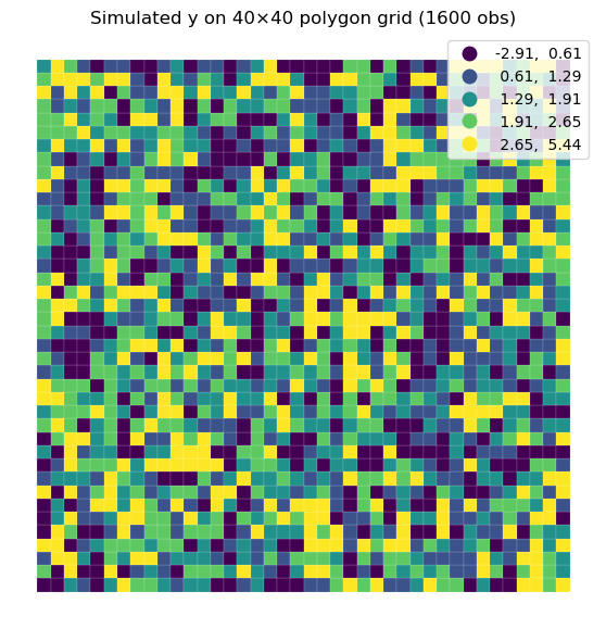
# Second Example: Larger 40×40 Grid (1600 obs)
# This benchmark repeats the backend comparison on a larger polygon grid.
gdf_full, y_full, X_full, W_full = simulate_sar_data(
    seed=PROFILE_CFG["seed"], n_side=40
)

gdf_full.plot(
    column="y",
    scheme="quantiles",
    cmap="viridis",
    legend=True,
    linewidth=0.1,
    edgecolor="white",
    figsize=(7, 7),
)
plt.title("Simulated y on 40×40 polygon grid (1600 obs)")
plt.axis("off")
plt.show()

rows_full = []
for backend_name in BACKENDS:
    print(f"Profiling backend={backend_name} on 40×40 grid...")
    rows_full.append(fit_backend(backend_name, y_full, X_full, W_full))

results_full = pd.DataFrame(rows_full)
results_full["rho_abs_error"] = (results_full["rho_hat"] - TRUE_RHO).abs()
results_full["beta_rmse"] = np.sqrt(
    (
        (
            results_full[["beta_0_hat", "beta_1_hat", "beta_2_hat"]].to_numpy()
            - TRUE_BETA[None, :]
        )
        ** 2
    ).mean(axis=1)
)
results_full = results_full.sort_values(
    ["available", "total_time_s"], ascending=[False, True], na_position="last"
).reset_index(drop=True)

display(
    results_full[display_cols].round(
        {"total_time_s": 3, "rho_hat": 3, "rho_abs_error": 3, "beta_rmse": 3}
    )
)
Profiling backend=c on 40×40 grid...
Profiling backend=numba on 40×40 grid...
Profiling backend=numpyro on 40×40 grid...
Profiling backend=blackjax on 40×40 grid...
Profiling backend=nutpie on 40×40 grid...
| backend | available | total_time_s | rho_hat | rho_abs_error | beta_rmse | divergences | error | |
|---|---|---|---|---|---|---|---|---|
| 0 | c | True | NaN | NaN | NaN | NaN | NaN | AttributeError: 'InferenceData' object has no ... |
| 1 | numba | True | NaN | NaN | NaN | NaN | NaN | AttributeError: 'InferenceData' object has no ... |
| 2 | numpyro | True | NaN | NaN | NaN | NaN | NaN | AttributeError: 'InferenceData' object has no ... |
| 3 | blackjax | True | NaN | NaN | NaN | NaN | NaN | AttributeError: 'InferenceData' object has no ... |
| 4 | nutpie | True | NaN | NaN | NaN | NaN | NaN | AttributeError: 'InferenceData' object has no ... |
ok_full = results_full[results_full["total_time_s"].notna()].copy()
fig, axes = plt.subplots(1, 2, figsize=(12, 4))

if not ok_full.empty:
    axes[0].bar(
        ok_full["backend"],
        ok_full["total_time_s"],
        color=["#4c78a8", "#f58518", "#54a24b", "#e45756"][: len(ok_full)],
    )
    axes[0].set_title("Total Runtime by Backend (40×40 grid)")
    axes[0].set_ylabel("seconds")

    axes[1].bar(
        ok_full["backend"],
        ok_full["rho_abs_error"],
        color=["#4c78a8", "#f58518", "#54a24b", "#e45756"][: len(ok_full)],
    )
    axes[1].set_title("Absolute Error in rho (40×40 grid)")
    axes[1].set_ylabel("|rho_hat - rho_true|")
else:
    axes[0].text(0.5, 0.5, "No successful backend runs", ha="center", va="center")
    axes[1].text(0.5, 0.5, "No successful backend runs", ha="center", va="center")
    axes[0].set_axis_off()
    axes[1].set_axis_off()

plt.tight_layout()
plt.show()
Reading The Results
Interpret the tables and plots with two constraints in mind:
these settings are still benchmark-sized, even on the larger 40×40 grid