Gibbs vs NUTS Profiling: Cross-Sectional Models
This notebook profiles the four Gaussian cross-sectional spatial models (SAR, SEM, SDM, SDEM) under both the NUTS and Gibbs sampling backends, comparing wall-clock time and posterior summary statistics.
Setup
NUTS: PyMC’s default NUTS sampler (via
nutpieorpymc)Gibbs (NumPy): 3-block Gibbs with adaptive slice sampling,
n_jobs=-1(parallel via joblib)Gibbs (JAX): 3-block Gibbs with MALA,
chain_method="vectorized"(JAX vmap)
All models use the same synthetic data generated from a 6×6 rook-contiguity lattice (n=49, k=3).
import time

import arviz as az
import numpy as np
import pandas as pd
from libpysal.graph import Graph

from neighbayes.models import SAR, SDEM, SDM, SEM

# Try importing JAX to check availability
try:
    import jax  # noqa: F401

    HAS_JAX = True
except ImportError:
    HAS_JAX = False

print(f"JAX available: {HAS_JAX}")
JAX available: True
1. Generate Synthetic Data
We use a 7×7 rook-contiguity lattice (n=49) with 3 regressors (intercept + 2 covariates). Each model type generates data from its own DGP so the spatial parameter is well-identified.
SIDE = 7  # 7x7 grid → n=49
SEED = 42
DRAWS = 2000
TUNE = 1000
CHAINS = 4


def make_rook_W(side: int) -> np.ndarray:
    """Row-standardized rook-contiguity weights on a side x side grid."""
    n = side * side
    W = np.zeros((n, n))
    for r in range(side):
        for c in range(side):
            i = r * side + c
            if r > 0:
                W[i, (r - 1) * side + c] = 1
            if r < side - 1:
                W[i, (r + 1) * side + c] = 1
            if c > 0:
                W[i, r * side + (c - 1)] = 1
            if c < side - 1:
                W[i, r * side + (c + 1)] = 1
    row_sums = W.sum(axis=1, keepdims=True)
    return W / np.where(row_sums == 0, 1, row_sums)


def W_to_graph(W_dense: np.ndarray) -> Graph:
    """Convert a dense weight matrix to a libpysal Graph."""
    n = W_dense.shape[0]
    focal, neighbor, weight = [], [], []
    for i in range(n):
        for j in range(n):
            if W_dense[i, j] != 0:
                focal.append(i)
                neighbor.append(j)
                weight.append(W_dense[i, j])
    return Graph.from_arrays(
        np.array(focal),
        np.array(neighbor),
        np.array(weight, dtype=float),
    ).transform("r")


W_dense = make_rook_W(SIDE)
W = W_to_graph(W_dense)
n = SIDE * SIDE
print(f"n = {n}, W shape = {W_dense.shape}")
n = 49, W shape = (49, 49)
from neighbayes.dgp.cross_sectional import (
    simulate_sar,
    simulate_sdem,
    simulate_sdm,
    simulate_sem,
)

rng = np.random.default_rng(SEED)

# SAR data
sar_out = simulate_sar(W=W_dense, rho=0.6, sigma=1.0, rng=rng)
y_sar, X_sar = sar_out["y"], sar_out["X"]

# SEM data
sem_out = simulate_sem(W=W_dense, lam=0.6, sigma=1.0, rng=rng)
y_sem, X_sem = sem_out["y"], sem_out["X"]

# SDM data
sdm_out = simulate_sdm(W=W_dense, rho=0.4, sigma=1.0, rng=rng)
y_sdm, X_sdm = sdm_out["y"], sdm_out["X"]

# SDEM data
sdem_out = simulate_sdem(W=W_dense, lam=0.4, sigma=1.0, rng=rng)
y_sdem, X_sdem = sdem_out["y"], sdem_out["X"]

print(f"SAR:  y={y_sar.shape}, X={X_sar.shape}")
print(f"SEM:  y={y_sem.shape}, X={X_sem.shape}")
print(f"SDM:  y={y_sdm.shape}, X={X_sdm.shape}")
print(f"SDEM: y={y_sdem.shape}, X={X_sdem.shape}")
SAR:  y=(49,), X=(49, 2)
SEM:  y=(49,), X=(49, 2)
SDM:  y=(49,), X=(49, 2)
SDEM: y=(49,), X=(49, 2)
2. Define the Profiling Function
We time each sampler configuration and collect:
Wall-clock time (seconds)
Posterior means for key parameters
R-hat and ESS diagnostics
def profile_model(model, sampler_config: dict, label: str) -> dict:
    """Fit a model with a given sampler config and return timing + diagnostics."""
    t0 = time.perf_counter()
    idata = model.fit(**sampler_config)
    elapsed = time.perf_counter() - t0

    # Extract spatial parameter name (rho for SAR/SDM, lam for SEM/SDEM)
    spatial_vars = [p for p in idata.posterior.data_vars if p in ("rho", "lam")]
    spatial_param = spatial_vars[0] if spatial_vars else None

    result = {
        "label": label,
        "elapsed_s": round(elapsed, 2),
    }

    # Posterior means (scalar parameters only)
    # beta is (chain, draw, k) — report intercept (first coefficient)
    result["intercept_mean"] = float(
        idata.posterior["beta"].mean(dim=["chain", "draw"]).values[0]
    )
    result["sigma_mean"] = float(idata.posterior["sigma"].mean())
    if spatial_param:
        result[f"{spatial_param}_mean"] = float(idata.posterior[spatial_param].mean())

    # Diagnostics — include all parameters for thorough R-hat / ESS checks
    diag_vars = ["beta", "sigma"] + ([spatial_param] if spatial_param else [])
    summary = az.summary(idata, var_names=diag_vars)
    result["rhat_max"] = round(float(summary["r_hat"].max()), 3)
    result["ess_bulk_min"] = int(summary["ess_bulk"].min())

    return result
3. Profile All Models
We profile each of the 4 models under 3 sampler configurations:
Config |
Backend |
Key settings |
|---|---|---|
NUTS |
PyMC NUTS |
|
Gibbs NumPy |
Slice sampling (adaptive) |
|
Gibbs JAX |
Slice sampling (JIT) |
|
COMMON = dict(
    draws=DRAWS, tune=TUNE, chains=CHAINS, random_seed=SEED, progressbar=False
)

configs = {
    "NUTS": dict(sampler="nuts", target_accept=0.9, **COMMON),
    "Gibbs-NumPy": dict(sampler="gibbs", gibbs_backend="numpy", n_jobs=-1, **COMMON),
}

if HAS_JAX:
    configs["Gibbs-JAX"] = dict(sampler="gibbs", gibbs_backend="jax", **COMMON)

print(f"Configs: {list(configs.keys())}")
Configs: ['NUTS', 'Gibbs-NumPy', 'Gibbs-JAX']
results = []

models_and_data = [
    ("SAR", SAR, y_sar, X_sar),
    ("SEM", SEM, y_sem, X_sem),
    ("SDM", SDM, y_sdm, X_sdm),
    ("SDEM", SDEM, y_sdem, X_sdem),
]

for model_name, ModelClass, y, X in models_and_data:
    print(f"\n{'=' * 60}")
    print(f"Model: {model_name}")
    print(f"{'=' * 60}")

    for config_name, config in configs.items():
        label = f"{model_name}/{config_name}"
        print(f"  Running {label}...", end=" ", flush=True)

        model = ModelClass(y=y, X=X, W=W)
        try:
            result = profile_model(model, config, label)
            print(
                f"{result['elapsed_s']:.1f}s  ρ̂={result.get('rho_mean', result.get('lam_mean', 'N/A')):.4f}  r̂={result['rhat_max']:.3f}  ESS={result['ess_bulk_min']}"
            )
        except Exception as e:
            result = {"label": label, "elapsed_s": None, "error": str(e)}
            print(f"FAILED: {e}")

        results.append(result)

print(f"\nDone! {len(results)} configurations profiled.")
============================================================
Model: SAR
============================================================
  Running SAR/NUTS...
16.0s  ρ̂=0.4057  r̂=1.000  ESS=4042
  Running SAR/Gibbs-NumPy...
3.3s  ρ̂=0.4173  r̂=1.000  ESS=7305
  Running SAR/Gibbs-JAX...
3.8s  ρ̂=0.4153  r̂=1.000  ESS=7136

============================================================
Model: SEM
============================================================
  Running SEM/NUTS...
16.3s  ρ̂=0.7646  r̂=1.000  ESS=3575
  Running SEM/Gibbs-NumPy...
4.5s  ρ̂=0.7861  r̂=1.000  ESS=7341
  Running SEM/Gibbs-JAX...
3.5s  ρ̂=0.7834  r̂=1.000  ESS=6907

============================================================
Model: SDM
============================================================
  Running SDM/NUTS...
14.2s  ρ̂=0.2812  r̂=1.000  ESS=3442
  Running SDM/Gibbs-NumPy...
3.8s  ρ̂=0.3030  r̂=1.000  ESS=6914
  Running SDM/Gibbs-JAX...
3.5s  ρ̂=0.2997  r̂=1.000  ESS=6814

============================================================
Model: SDEM
============================================================
  Running SDEM/NUTS...
14.0s  ρ̂=0.4472  r̂=1.000  ESS=5180
  Running SDEM/Gibbs-NumPy...
4.9s  ρ̂=0.4801  r̂=1.000  ESS=7280
  Running SDEM/Gibbs-JAX...
3.7s  ρ̂=0.4769  r̂=1.000  ESS=6771

Done! 12 configurations profiled.
Initializing NUTS using jitter+adapt_diag...
Multiprocess sampling (4 chains in 2 jobs)
NUTS: [rho, beta, sigma2]
Sampling 4 chains for 1_000 tune and 2_000 draw iterations (4_000 + 8_000 draws total) took 12 seconds.
/home/runner/micromamba/envs/test/lib/python3.14/site-packages/neighbayes/_logdet/_jax.py:188: ComplexWarning: Casting complex values to real discards the imaginary part
  W_arr = np.asarray(W, dtype=np.float64)
Initializing NUTS using jitter+adapt_diag...
Multiprocess sampling (4 chains in 2 jobs)
NUTS: [lam, beta, sigma2]
Sampling 4 chains for 1_000 tune and 2_000 draw iterations (4_000 + 8_000 draws total) took 11 seconds.
/home/runner/micromamba/envs/test/lib/python3.14/site-packages/neighbayes/_logdet/_jax.py:188: ComplexWarning: Casting complex values to real discards the imaginary part
  W_arr = np.asarray(W, dtype=np.float64)
Initializing NUTS using jitter+adapt_diag...
Multiprocess sampling (4 chains in 2 jobs)
NUTS: [rho, beta, sigma2]
Sampling 4 chains for 1_000 tune and 2_000 draw iterations (4_000 + 8_000 draws total) took 12 seconds.
/home/runner/micromamba/envs/test/lib/python3.14/site-packages/neighbayes/_logdet/_jax.py:188: ComplexWarning: Casting complex values to real discards the imaginary part
  W_arr = np.asarray(W, dtype=np.float64)
Initializing NUTS using jitter+adapt_diag...
Multiprocess sampling (4 chains in 2 jobs)
NUTS: [lam, beta, sigma2]
Sampling 4 chains for 1_000 tune and 2_000 draw iterations (4_000 + 8_000 draws total) took 11 seconds.
/home/runner/micromamba/envs/test/lib/python3.14/site-packages/neighbayes/_logdet/_jax.py:188: ComplexWarning: Casting complex values to real discards the imaginary part
  W_arr = np.asarray(W, dtype=np.float64)
4. Results Summary
# Build a clean results DataFrame
rows = []
for r in results:
    if "error" in r:
        rows.append(
            {"Model/Sampler": r["label"], "Time (s)": None, "Error": r["error"]}
        )
        continue
    model_name, config_name = r["label"].split("/")
    spatial_key = (
        "rho_mean" if "rho_mean" in r else ("lam_mean" if "lam_mean" in r else None)
    )
    rows.append(
        {
            "Model": model_name,
            "Sampler": config_name,
            "Time (s)": r["elapsed_s"],
            "Intercept": round(r["intercept_mean"], 4),
            "σ̂": round(r["sigma_mean"], 4),
            "ρ̂/λ̂": round(r.get(spatial_key, float("nan")), 4) if spatial_key else None,
            "max R̂": r["rhat_max"],
            "min ESS": r["ess_bulk_min"],
        }
    )

df = pd.DataFrame(rows)
# Drop duplicates in case cells were re-run
df = df.drop_duplicates(subset=["Model", "Sampler"], keep="last")
df.style.format(
    {"Time (s)": "{:.1f}", "Intercept": "{:.4f}", "σ̂": "{:.4f}", "ρ̂/λ̂": "{:.4f}"}
)
| Model | Sampler | Time (s) | Intercept | σ̂ | ρ̂/λ̂ | max R̂ | min ESS | |
|---|---|---|---|---|---|---|---|---|
| 0 | SAR | NUTS | 16.0 | 1.3207 | 0.8343 | 0.4057 | 1.000000 | 4042 |
| 1 | SAR | Gibbs-NumPy | 3.3 | 1.2924 | 0.8344 | 0.4173 | 1.000000 | 7305 |
| 2 | SAR | Gibbs-JAX | 3.8 | 1.2972 | 0.8360 | 0.4153 | 1.000000 | 7136 |
| 3 | SEM | NUTS | 16.3 | 1.0499 | 0.9325 | 0.7646 | 1.000000 | 3575 |
| 4 | SEM | Gibbs-NumPy | 4.5 | 1.0426 | 0.9250 | 0.7861 | 1.000000 | 7341 |
| 5 | SEM | Gibbs-JAX | 3.5 | 1.0369 | 0.9290 | 0.7834 | 1.000000 | 6907 |
| 6 | SDM | NUTS | 14.2 | 1.2825 | 1.1647 | 0.2812 | 1.000000 | 3442 |
| 7 | SDM | Gibbs-NumPy | 3.8 | 1.2531 | 1.1624 | 0.3030 | 1.000000 | 6914 |
| 8 | SDM | Gibbs-JAX | 3.5 | 1.2568 | 1.1631 | 0.2997 | 1.000000 | 6814 |
| 9 | SDEM | NUTS | 14.0 | 1.0022 | 1.1653 | 0.4472 | 1.000000 | 5180 |
| 10 | SDEM | Gibbs-NumPy | 4.9 | 0.9902 | 1.1591 | 0.4801 | 1.000000 | 7280 |
| 11 | SDEM | Gibbs-JAX | 3.7 | 0.9943 | 1.1624 | 0.4769 | 1.000000 | 6771 |
5. Speedup Comparison
How much faster is Gibbs compared to NUTS for each model?
# Pivot to compare times (use drop_duplicates to guard against re-runs)
if len(df) > 0 and "Time (s)" in df.columns:
    pivot = df.drop_duplicates(subset=["Model", "Sampler"], keep="last").pivot(
        index="Model", columns="Sampler", values="Time (s)"
    )
    if "NUTS" in pivot.columns:
        for col in pivot.columns:
            if col != "NUTS":
                pivot[f"{col}/NUTS"] = pivot[col] / pivot["NUTS"]
        print("Time relative to NUTS (< 1 means faster):")
        speedup_cols = [c for c in pivot.columns if "/NUTS" in c]
        display(
            pivot[
                ["NUTS"]
                + [c for c in pivot.columns if c != "NUTS" and "/NUTS" not in c]
                + speedup_cols
            ].round(2)
        )
    else:
        display(pivot.round(2))
else:
    print("No results to display.")
Time relative to NUTS (< 1 means faster):
| Sampler | NUTS | Gibbs-JAX | Gibbs-NumPy | Gibbs-JAX/NUTS | Gibbs-NumPy/NUTS |
|---|---|---|---|---|---|
| Model | |||||
| SAR | 15.99 | 3.84 | 3.31 | 0.24 | 0.21 |
| SDEM | 13.98 | 3.72 | 4.90 | 0.27 | 0.35 |
| SDM | 14.25 | 3.45 | 3.81 | 0.24 | 0.27 |
| SEM | 16.33 | 3.49 | 4.51 | 0.21 | 0.28 |
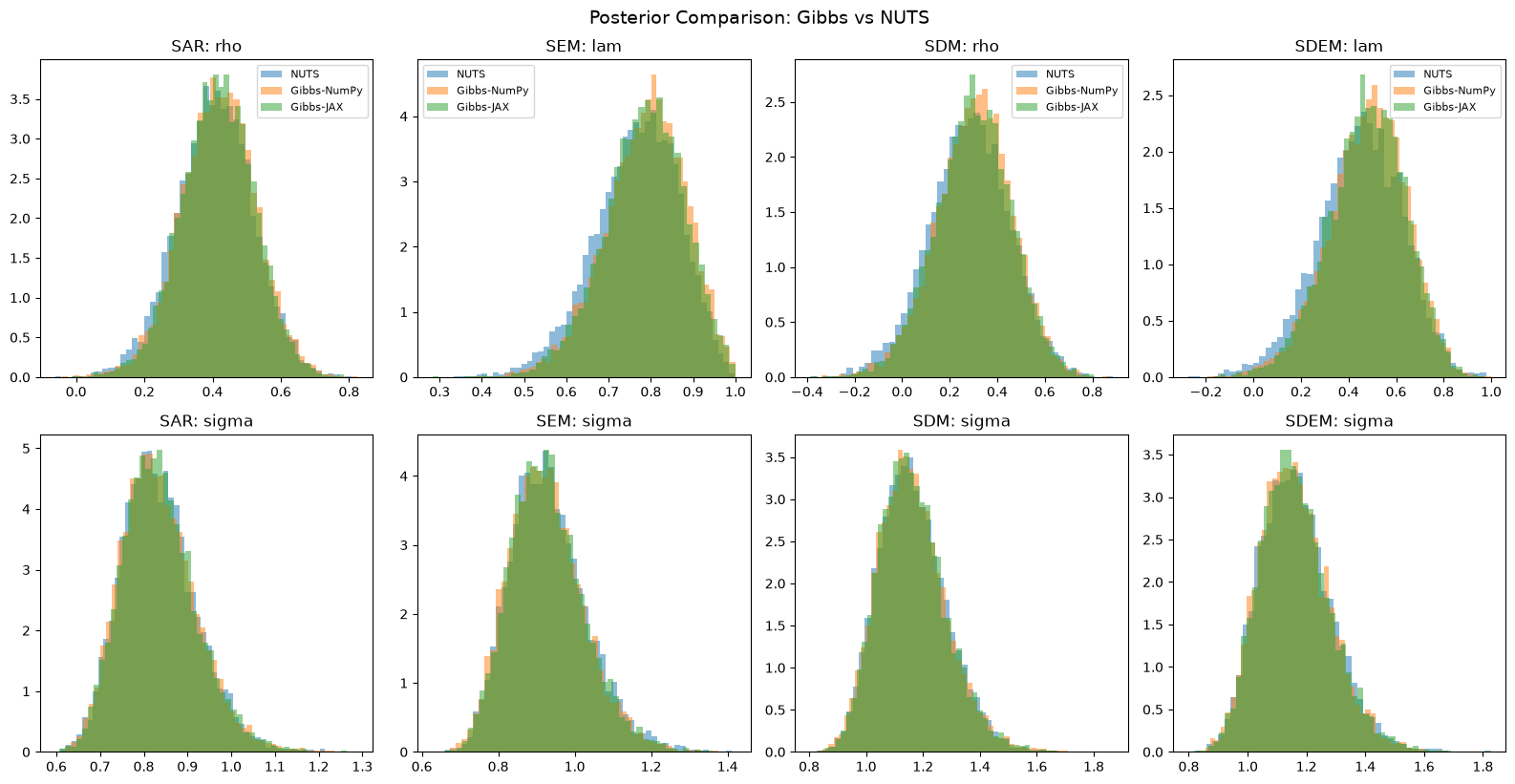
6. Posterior Comparison
Compare posterior distributions across samplers for each model. The Gibbs and NUTS posteriors should agree closely for well-identified parameters.
import matplotlib.pyplot as plt

# Re-fit all models and store idatas for comparison plots
idatas = {}
for model_name, ModelClass, y, X in models_and_data:
    idatas[model_name] = {}
    for config_name, config in configs.items():
        label = f"{model_name}/{config_name}"
        model = ModelClass(y=y, X=X, W=W)
        try:
            idata = model.fit(**config)
            idatas[model_name][config_name] = idata
        except Exception:
            pass

# Plot comparison for each model
spatial_param_map = {"SAR": "rho", "SEM": "lam", "SDM": "rho", "SDEM": "lam"}

fig, axes = plt.subplots(2, 4, figsize=(16, 8))

for col, model_name in enumerate(["SAR", "SEM", "SDM", "SDEM"]):
    param = spatial_param_map[model_name]
    for row, param_name in enumerate([param, "sigma"]):
        ax = axes[row, col]
        for config_name in configs:
            if config_name in idatas.get(model_name, {}):
                idata = idatas[model_name][config_name]
                samples = idata.posterior[param_name].values.flatten()
                ax.hist(samples, bins=50, alpha=0.5, density=True, label=config_name)
        ax.set_title(f"{model_name}: {param_name}")
        if row == 0:
            ax.legend(fontsize=8)

plt.tight_layout()
plt.suptitle("Posterior Comparison: Gibbs vs NUTS", y=1.02, fontsize=14)
plt.show()
Initializing NUTS using jitter+adapt_diag...
Multiprocess sampling (4 chains in 2 jobs)
NUTS: [rho, beta, sigma2]
Sampling 4 chains for 1_000 tune and 2_000 draw iterations (4_000 + 8_000 draws total) took 12 seconds.
/home/runner/micromamba/envs/test/lib/python3.14/site-packages/neighbayes/_logdet/_jax.py:188: ComplexWarning: Casting complex values to real discards the imaginary part
  W_arr = np.asarray(W, dtype=np.float64)
Initializing NUTS using jitter+adapt_diag...
Multiprocess sampling (4 chains in 2 jobs)
NUTS: [lam, beta, sigma2]
Sampling 4 chains for 1_000 tune and 2_000 draw iterations (4_000 + 8_000 draws total) took 12 seconds.
/home/runner/micromamba/envs/test/lib/python3.14/site-packages/neighbayes/_logdet/_jax.py:188: ComplexWarning: Casting complex values to real discards the imaginary part
  W_arr = np.asarray(W, dtype=np.float64)
Initializing NUTS using jitter+adapt_diag...
Multiprocess sampling (4 chains in 2 jobs)
NUTS: [rho, beta, sigma2]
Sampling 4 chains for 1_000 tune and 2_000 draw iterations (4_000 + 8_000 draws total) took 12 seconds.
/home/runner/micromamba/envs/test/lib/python3.14/site-packages/neighbayes/_logdet/_jax.py:188: ComplexWarning: Casting complex values to real discards the imaginary part
  W_arr = np.asarray(W, dtype=np.float64)
Initializing NUTS using jitter+adapt_diag...
Multiprocess sampling (4 chains in 2 jobs)
NUTS: [lam, beta, sigma2]
Sampling 4 chains for 1_000 tune and 2_000 draw iterations (4_000 + 8_000 draws total) took 11 seconds.
/home/runner/micromamba/envs/test/lib/python3.14/site-packages/neighbayes/_logdet/_jax.py:188: ComplexWarning: Casting complex values to real discards the imaginary part
  W_arr = np.asarray(W, dtype=np.float64)
6b. Diagnostics: Gibbs Mixing for SEM/SDEM
The Gibbs sampler now uses collapsed updates for all spatial parameters:
SAR/SDM: Collapsed update for ρ — integrates out β and σ² analytically, giving a marginal density
log p(ρ | y)that doesn’t depend on current β and σ² draws. This produces excellent mixing.SEM/SDEM: Collapsed update for λ — also integrates out β and σ² analytically. The collapsed density includes an extra Jacobian term
-(1/2)log|X*^T X*|because the transformed design matrix X* = (I - λW)X depends on λ (unlike SAR where X is fixed).
The cell below compares trace plots and posterior summaries for the spatial parameter across samplers.
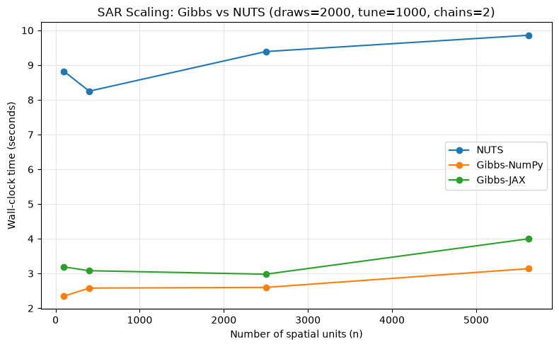
7. Scaling: Effect of n on Gibbs vs NUTS Time
How does wall-clock time scale with the number of spatial units?
SCALE_DRAWS = 2000
SCALE_TUNE = 1000
SCALE_CHAINS = 2
SIDES = [10, 20, 50, 75]  # n = 16, 36, 64, 100

scale_results = []

scale_configs = {
    "NUTS": dict(
        sampler="nuts",
        target_accept=0.9,
        draws=SCALE_DRAWS,
        tune=SCALE_TUNE,
        chains=SCALE_CHAINS,
        random_seed=SEED,
        progressbar=False,
    ),
    "Gibbs-NumPy": dict(
        sampler="gibbs",
        gibbs_backend="numpy",
        n_jobs=-1,
        draws=SCALE_DRAWS,
        tune=SCALE_TUNE,
        chains=SCALE_CHAINS,
        random_seed=SEED,
        progressbar=False,
    ),
}
if HAS_JAX:
    scale_configs["Gibbs-JAX"] = dict(
        sampler="gibbs",
        gibbs_backend="jax",
        draws=SCALE_DRAWS,
        tune=SCALE_TUNE,
        chains=SCALE_CHAINS,
        random_seed=SEED,
        progressbar=False,
    )
    scale_configs["NUTS-JAX"] = dict(
        sampler="nuts",
        gibbs_backend="jax",
        draws=SCALE_DRAWS,
        tune=SCALE_TUNE,
        chains=SCALE_CHAINS,
        random_seed=SEED,
        progressbar=False,
        nuts_sampler="blackjax",
    )

for side in SIDES:
    n = side * side
    W_dense_s = make_rook_W(side)
    W_s = W_to_graph(W_dense_s)
    rng_s = np.random.default_rng(SEED)
    out_s = simulate_sar(W=W_dense_s, rho=0.5, sigma=1.0, rng=rng_s)
    y_s, X_s = out_s["y"], out_s["X"]

    print(f"\nn = {n} (side={side})")
    for config_name, config in scale_configs.items():
        label = f"n={n}/{config_name}"
        model = SAR(y=y_s, X=X_s, W=W_s)
        try:
            result = profile_model(model, config, label)
            print(f"  {config_name}: {result['elapsed_s']:.1f}s")
            result["n"] = n
            result["sampler"] = config_name
            scale_results.append(result)
        except Exception as e:
            print(f"  {config_name}: FAILED ({e})")

print("\nScaling benchmark complete.")
n = 100 (side=10)
  NUTS: 8.8s
  Gibbs-NumPy: 2.4s
  Gibbs-JAX: 3.2s
  NUTS-JAX: FAILED (build_kernel.<locals>.kernel() got an unexpected keyword argument 'progress_bar')

n = 400 (side=20)
  NUTS: 8.2s
  Gibbs-NumPy: 2.6s
  Gibbs-JAX: 3.1s
  NUTS-JAX: FAILED (build_kernel.<locals>.kernel() got an unexpected keyword argument 'progress_bar')

n = 2500 (side=50)
  NUTS: 9.4s
  Gibbs-NumPy: 2.6s
  Gibbs-JAX: 3.0s
  NUTS-JAX: FAILED (build_kernel.<locals>.kernel() got an unexpected keyword argument 'progress_bar')

n = 5625 (side=75)
  NUTS: 9.9s
  Gibbs-NumPy: 3.1s
  Gibbs-JAX: 4.0s
  NUTS-JAX: FAILED (build_kernel.<locals>.kernel() got an unexpected keyword argument 'progress_bar')

Scaling benchmark complete.
Initializing NUTS using jitter+adapt_diag...
Multiprocess sampling (2 chains in 2 jobs)
NUTS: [rho, beta, sigma2]
Sampling 2 chains for 1_000 tune and 2_000 draw iterations (2_000 + 4_000 draws total) took 6 seconds.
We recommend running at least 4 chains for robust computation of convergence diagnostics
/home/runner/micromamba/envs/test/lib/python3.14/site-packages/neighbayes/_logdet/_jax.py:188: ComplexWarning: Casting complex values to real discards the imaginary part
  W_arr = np.asarray(W, dtype=np.float64)
/home/runner/micromamba/envs/test/lib/python3.14/site-packages/tqdm/auto.py:21: TqdmWarning: IProgress not found. Please update jupyter and ipywidgets. See https://ipywidgets.readthedocs.io/en/stable/user_install.html
  from .autonotebook import tqdm as notebook_tqdm
Initializing NUTS using jitter+adapt_diag...
Multiprocess sampling (2 chains in 2 jobs)
NUTS: [rho, beta, sigma2]
Sampling 2 chains for 1_000 tune and 2_000 draw iterations (2_000 + 4_000 draws total) took 6 seconds.
We recommend running at least 4 chains for robust computation of convergence diagnostics
/home/runner/micromamba/envs/test/lib/python3.14/site-packages/neighbayes/_logdet/_jax.py:188: ComplexWarning: Casting complex values to real discards the imaginary part
  W_arr = np.asarray(W, dtype=np.float64)
Initializing NUTS using jitter+adapt_diag...
Multiprocess sampling (2 chains in 2 jobs)
NUTS: [rho, beta, sigma2]
Sampling 2 chains for 1_000 tune and 2_000 draw iterations (2_000 + 4_000 draws total) took 7 seconds.
We recommend running at least 4 chains for robust computation of convergence diagnostics
Initializing NUTS using jitter+adapt_diag...
Multiprocess sampling (2 chains in 2 jobs)
NUTS: [rho, beta, sigma2]
Sampling 2 chains for 1_000 tune and 2_000 draw iterations (2_000 + 4_000 draws total) took 7 seconds.
We recommend running at least 4 chains for robust computation of convergence diagnostics
# Plot scaling results
if scale_results:
    scale_df = pd.DataFrame(scale_results)
    fig, ax = plt.subplots(figsize=(8, 5))
    for sampler in scale_df["sampler"].unique():
        sub = scale_df[scale_df["sampler"] == sampler].sort_values("n")
        ax.plot(sub["n"], sub["elapsed_s"], marker="o", label=sampler)
    ax.set_xlabel("Number of spatial units (n)")
    ax.set_ylabel("Wall-clock time (seconds)")
    ax.set_title(
        f"SAR Scaling: Gibbs vs NUTS (draws={SCALE_DRAWS}, tune={SCALE_TUNE}, chains={SCALE_CHAINS})"
    )
    ax.legend()
    ax.grid(True, alpha=0.3)
    plt.tight_layout()
    plt.show()
else:
    print("No scaling results to plot.")
SCALE_DRAWS = 2000
SCALE_TUNE = 1000
SCALE_CHAINS = 2
SIDES = [10, 20, 50, 75]  # n = 16, 36, 64, 100

scale_results = []

scale_configs = {
    "NUTS": dict(
        sampler="nuts",
        target_accept=0.9,
        draws=SCALE_DRAWS,
        tune=SCALE_TUNE,
        chains=SCALE_CHAINS,
        random_seed=SEED,
        progressbar=False,
    ),
    "Gibbs-NumPy": dict(
        sampler="gibbs",
        gibbs_backend="numpy",
        n_jobs=-1,
        draws=SCALE_DRAWS,
        tune=SCALE_TUNE,
        chains=SCALE_CHAINS,
        random_seed=SEED,
        progressbar=False,
    ),
}
if HAS_JAX:
    scale_configs["Gibbs-JAX"] = dict(
        sampler="gibbs",
        gibbs_backend="jax",
        draws=SCALE_DRAWS,
        tune=SCALE_TUNE,
        chains=SCALE_CHAINS,
        random_seed=SEED,
        progressbar=False,
    )
    scale_configs["NUTS-JAX"] = dict(
        sampler="nuts",
        gibbs_backend="jax",
        draws=SCALE_DRAWS,
        tune=SCALE_TUNE,
        chains=SCALE_CHAINS,
        random_seed=SEED,
        progressbar=False,
        nuts_sampler="blackjax",
    )

for side in SIDES:
    n = side * side
    W_dense_s = make_rook_W(side)
    W_s = W_to_graph(W_dense_s)
    rng_s = np.random.default_rng(SEED)
    out_s = simulate_sem(W=W_dense_s, lam=0.5, sigma=1.0, rng=rng_s)
    y_s, X_s = out_s["y"], out_s["X"]

    print(f"\nn = {n} (side={side})")
    for config_name, config in scale_configs.items():
        label = f"n={n}/{config_name}"
        model = SEM(y=y_s, X=X_s, W=W_s)
        try:
            result = profile_model(model, config, label)
            print(f"  {config_name}: {result['elapsed_s']:.1f}s")
            result["n"] = n
            result["sampler"] = config_name
            scale_results.append(result)
        except Exception as e:
            print(f"  {config_name}: FAILED ({e})")

print("\nScaling benchmark complete.")
n = 100 (side=10)
  NUTS: 8.3s
  Gibbs-NumPy: 3.0s
  Gibbs-JAX: 3.2s
  NUTS-JAX: FAILED (build_kernel.<locals>.kernel() got an unexpected keyword argument 'progress_bar')

n = 400 (side=20)
  NUTS: 8.6s
  Gibbs-NumPy: 3.0s
  Gibbs-JAX: 3.3s
  NUTS-JAX: FAILED (build_kernel.<locals>.kernel() got an unexpected keyword argument 'progress_bar')

n = 2500 (side=50)
  NUTS: 9.5s
  Gibbs-NumPy: 3.2s
  Gibbs-JAX: 3.3s
  NUTS-JAX: FAILED (build_kernel.<locals>.kernel() got an unexpected keyword argument 'progress_bar')

n = 5625 (side=75)
  NUTS: 10.7s
  Gibbs-NumPy: 3.7s
  Gibbs-JAX: 3.4s
  NUTS-JAX: FAILED (build_kernel.<locals>.kernel() got an unexpected keyword argument 'progress_bar')

Scaling benchmark complete.
Initializing NUTS using jitter+adapt_diag...
Multiprocess sampling (2 chains in 2 jobs)
NUTS: [lam, beta, sigma2]
Sampling 2 chains for 1_000 tune and 2_000 draw iterations (2_000 + 4_000 draws total) took 6 seconds.
We recommend running at least 4 chains for robust computation of convergence diagnostics
/home/runner/micromamba/envs/test/lib/python3.14/site-packages/neighbayes/_logdet/_jax.py:188: ComplexWarning: Casting complex values to real discards the imaginary part
  W_arr = np.asarray(W, dtype=np.float64)
Initializing NUTS using jitter+adapt_diag...
Multiprocess sampling (2 chains in 2 jobs)
NUTS: [lam, beta, sigma2]
Sampling 2 chains for 1_000 tune and 2_000 draw iterations (2_000 + 4_000 draws total) took 6 seconds.
We recommend running at least 4 chains for robust computation of convergence diagnostics
/home/runner/micromamba/envs/test/lib/python3.14/site-packages/neighbayes/_logdet/_jax.py:188: ComplexWarning: Casting complex values to real discards the imaginary part
  W_arr = np.asarray(W, dtype=np.float64)
Initializing NUTS using jitter+adapt_diag...
Multiprocess sampling (2 chains in 2 jobs)
NUTS: [lam, beta, sigma2]
Sampling 2 chains for 1_000 tune and 2_000 draw iterations (2_000 + 4_000 draws total) took 7 seconds.
We recommend running at least 4 chains for robust computation of convergence diagnostics
Initializing NUTS using jitter+adapt_diag...
Multiprocess sampling (2 chains in 2 jobs)
NUTS: [lam, beta, sigma2]
Sampling 2 chains for 1_000 tune and 2_000 draw iterations (2_000 + 4_000 draws total) took 8 seconds.
We recommend running at least 4 chains for robust computation of convergence diagnostics
# Plot scaling results
if scale_results:
    scale_df = pd.DataFrame(scale_results)
    fig, ax = plt.subplots(figsize=(8, 5))
    for sampler in scale_df["sampler"].unique():
        sub = scale_df[scale_df["sampler"] == sampler].sort_values("n")
        ax.plot(sub["n"], sub["elapsed_s"], marker="o", label=sampler)
    ax.set_xlabel("Number of spatial units (n)")
    ax.set_ylabel("Wall-clock time (seconds)")
    ax.set_title(
        f"SAR Scaling: Gibbs vs NUTS (draws={SCALE_DRAWS}, tune={SCALE_TUNE}, chains={SCALE_CHAINS})"
    )
    ax.legend()
    ax.grid(True, alpha=0.3)
    plt.tight_layout()
    plt.show()
else:
    print("No scaling results to plot.")
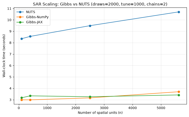
Gibbs is way faster with better ESS than NUTS. The JAX-based Gibbs sampler wins across the board in time/ESS tradeoff.