JAX vs NumPy Gibbs Profiling: Logit & Negbin¶

This notebook profiles the JAX and NumPy Gibbs samplers for SAR-logit, SEM-logit, and SAR-Negative Binomial models, comparing wall-clock time, ESS, and posterior agreement.

Architecture¶

Both backends use the same Gibbs structure (PG ω → ρ → β → α), but differ in the linear algebra and ρ-update strategy:

Backend	ρ/λ update	Linear algebra	Key advantage
Gibbs-NumPy (`gibbs_backend="numpy"`)	Slice + Krylov	CHOLMOD/CG sparse solves	Process-level chain parallelism via `joblib`
Gibbs-JAX (`gibbs_backend="jax"`)	Slice (all models)	Sparse solves via `sparsax`	Whole sweep JIT-compiled into one XLA kernel

Model-specific ρ/λ strategies¶

SAR/SEM-Logit (JAX): Stepping-out + shrinkage slice sampling on the collapsed log-density. Each candidate needs only a forward density evaluation — no gradient required. This avoids the O(n³) forward + O(n³) backward cost of jax.value_and_grad through jnp.linalg.solve that made MALA 3.6× slower than NumPy.
SAR-NB reduced form (both backends): Slice sampling with a shift-invert Krylov basis. The β-marginalised density needs \(U = (I-\rho W)^{-1}X\); the Krylov basis builds U(ρ) as a Horner polynomial in Δρ, giving O(m·n·k) per candidate.

import time

import arviz as az
import matplotlib.pyplot as plt
import numpy as np
import pandas as pd
from libpysal.graph import Graph

from neighbayes.dgp import simulate_sar_logit, simulate_sar_negbin, simulate_sem_logit
from neighbayes.models import SARLogit, SARNegBin, SEMLogit

try:
    import jax

    # Clear JAX JIT cache so code changes take effect without kernel restart
    jax.clear_caches()
    HAS_JAX = True
except ImportError:
    HAS_JAX = False

print(f"JAX available: {HAS_JAX}")

JAX available: True

/home/runner/micromamba/envs/test/lib/python3.14/site-packages/tqdm/auto.py:21: TqdmWarning: IProgress not found. Please update jupyter and ipywidgets. See https://ipywidgets.readthedocs.io/en/stable/user_install.html
  from .autonotebook import tqdm as notebook_tqdm

1. Generate Synthetic Data¶

We use a 7×7 rook-contiguity lattice (n=49) with 3 regressors. Each model type generates data from its own DGP so the spatial parameter is well-identified.

SIDE = 7  # 7x7 grid → n=49
SEED = 42
DRAWS = 2000
TUNE = 1000
CHAINS = 4


def make_rook_W(side: int) -> np.ndarray:
    """Row-standardized rook-contiguity weights on a side x side grid."""
    n = side * side
    W = np.zeros((n, n))
    for r in range(side):
        for c in range(side):
            i = r * side + c
            if r > 0:
                W[i, (r - 1) * side + c] = 1
            if r < side - 1:
                W[i, (r + 1) * side + c] = 1
            if c > 0:
                W[i, r * side + (c - 1)] = 1
            if c < side - 1:
                W[i, r * side + (c + 1)] = 1
    row_sums = W.sum(axis=1, keepdims=True)
    return W / np.where(row_sums == 0, 1, row_sums)


def W_to_graph(W_dense: np.ndarray) -> Graph:
    """Convert a dense weight matrix to a libpysal Graph."""
    n = W_dense.shape[0]
    focal, neighbor, weight = [], [], []
    for i in range(n):
        for j in range(n):
            if W_dense[i, j] != 0:
                focal.append(i)
                neighbor.append(j)
                weight.append(W_dense[i, j])
    return Graph.from_arrays(
        np.array(focal),
        np.array(neighbor),
        np.array(weight, dtype=float),
    ).transform("r")


W_dense = make_rook_W(SIDE)
W = W_to_graph(W_dense)
n = SIDE * SIDE
print(f"n = {n}, W shape = {W_dense.shape}")

n = 49, W shape = (49, 49)

rng = np.random.default_rng(SEED)

# SAR-logit data
sar_logit_out = simulate_sar_logit(W=W_dense, rho=0.6, rng=rng)
y_sar_logit, X_sar_logit = sar_logit_out["y"], sar_logit_out["X"]

# SEM-logit data
sem_logit_out = simulate_sem_logit(W=W_dense, lam=0.6, rng=rng)
y_sem_logit, X_sem_logit = sem_logit_out["y"], sem_logit_out["X"]

# SAR-NB data
sar_nb_out = simulate_sar_negbin(
    n=n, rho=0.5, beta=np.array([2.0, 1.0, -0.5]), alpha=5.0, rng=rng, W=W_dense
)
y_sar_nb, X_sar_nb = sar_nb_out["y"], sar_nb_out["X"]

print(f"SAR-logit: y={y_sar_logit.shape}, X={X_sar_logit.shape}")
print(f"SEM-logit: y={y_sem_logit.shape}, X={X_sem_logit.shape}")
print(f"SAR-NB:    y={y_sar_nb.shape}, X={X_sar_nb.shape}")

SAR-logit: y=(49,), X=(49, 2)
SEM-logit: y=(49,), X=(49, 2)
SAR-NB:    y=(49,), X=(49, 3)

2. Define the Profiling Function¶

We time each sampler configuration and collect:

Wall-clock time (seconds)
Posterior means for key parameters
R-hat and ESS diagnostics

def profile_model(model, sampler_config: dict, label: str) -> dict:
    """Fit a model with a given sampler config and return timing + diagnostics."""
    t0 = time.perf_counter()
    idata = model.fit(**sampler_config)
    elapsed = time.perf_counter() - t0

    # Extract spatial parameter name (rho for SAR, lam for SEM)
    spatial_vars = [p for p in idata.posterior.data_vars if p in ("rho", "lam")]
    spatial_param = spatial_vars[0] if spatial_vars else None

    result = {
        "label": label,
        "elapsed_s": round(elapsed, 2),
    }

    # Posterior means
    result["intercept_mean"] = float(
        idata.posterior["beta"].mean(dim=["chain", "draw"]).values[0]
    )
    if spatial_param:
        result[f"{spatial_param}_mean"] = float(idata.posterior[spatial_param].mean())

    # For NB, also report alpha and sigma
    if "alpha" in idata.posterior.data_vars:
        result["alpha_mean"] = float(idata.posterior["alpha"].mean())
    if "sigma" in idata.posterior.data_vars:
        result["sigma_mean"] = float(idata.posterior["sigma"].mean())

    # Diagnostics
    diag_vars = ["beta"] + ([spatial_param] if spatial_param else [])
    if "alpha" in idata.posterior.data_vars:
        diag_vars.append("alpha")
    if "sigma" in idata.posterior.data_vars:
        diag_vars.append("sigma")
    summary = az.summary(idata, var_names=diag_vars)
    result["rhat_max"] = round(float(summary["r_hat"].max()), 3)
    result["ess_bulk_min"] = int(summary["ess_bulk"].min())

    return result

3. Profile All Models¶

We profile each of the 3 models under 2 Gibbs configurations:

Config	Backend	ρ/λ update	Linear algebra
Gibbs-NumPy	`"numpy"`	Slice + Krylov	CHOLMOD/CG sparse
Gibbs-JAX	`"jax"`	Slice (all models)	`sparsax` sparse (dense fallback)

COMMON = dict(
    draws=DRAWS, tune=TUNE, chains=CHAINS, random_seed=SEED, progressbar=False
)

configs = {
    "Gibbs-NumPy": dict(sampler="gibbs", gibbs_backend="numpy", n_jobs=-1, **COMMON),
}

if HAS_JAX:
    configs["Gibbs-JAX"] = dict(sampler="gibbs", gibbs_backend="jax", **COMMON)

print(f"Configs: {list(configs.keys())}")

Configs: ['Gibbs-NumPy', 'Gibbs-JAX']

results = []

models_and_data = [
    ("SAR-Logit", SARLogit, y_sar_logit, X_sar_logit),
    ("SEM-Logit", SEMLogit, y_sem_logit, X_sem_logit),
    ("SAR-NB", SARNegBin, y_sar_nb, X_sar_nb),
]

for model_name, ModelClass, y, X in models_and_data:
    print(f"\n{'=' * 60}")
    print(f"Model: {model_name}")
    print(f"{'=' * 60}")

    for config_name, config in configs.items():
        label = f"{model_name}/{config_name}"
        print(f"  Running {label}...", end=" ", flush=True)

        model = ModelClass(y=y, X=X, W=W)
        try:
            result = profile_model(model, config, label)
            spatial_key = (
                "rho_mean"
                if "rho_mean" in result
                else ("lam_mean" if "lam_mean" in result else None)
            )
            spatial_val = result.get(spatial_key, "N/A")
            if isinstance(spatial_val, float):
                spatial_val = f"{spatial_val:.4f}"
            print(
                f"{result['elapsed_s']:.1f}s  ρ̂/λ̂={spatial_val}  r̂={result['rhat_max']:.3f}  ESS={result['ess_bulk_min']}"
            )
        except Exception as e:
            result = {"label": label, "elapsed_s": None, "error": str(e)}
            print(f"FAILED: {e}")

        results.append(result)

print(f"\nDone! {len(results)} configurations profiled.")

============================================================
Model: SAR-Logit
============================================================
  Running SAR-Logit/Gibbs-NumPy...
11.1s  ρ̂/λ̂=-0.1344  r̂=1.000  ESS=4495
  Running SAR-Logit/Gibbs-JAX...
2.7s  ρ̂/λ̂=-0.1303  r̂=1.000  ESS=4793

============================================================
Model: SEM-Logit
============================================================
  Running SEM-Logit/Gibbs-NumPy...
17.1s  ρ̂/λ̂=0.0512  r̂=1.010  ESS=638
  Running SEM-Logit/Gibbs-JAX...
2.1s  ρ̂/λ̂=0.0468  r̂=1.010  ESS=666

============================================================
Model: SAR-NB
============================================================
  Running SAR-NB/Gibbs-NumPy...
10.6s  ρ̂/λ̂=0.4288  r̂=1.000  ESS=1217
  Running SAR-NB/Gibbs-JAX...
2.5s  ρ̂/λ̂=0.4235  r̂=1.000  ESS=1204

Done! 6 configurations profiled.

/home/runner/micromamba/envs/test/lib/python3.14/site-packages/neighbayes/samplers/negbin_reduced/__init__.py:85: UserWarning: SAR Negative Binomial models require large samples for reliable spatial parameter recovery. With n=49, posterior estimates of ρ and α may be severely attenuated. n ≥ 900 is recommended.
  return model._fit_gibbs(
/home/runner/micromamba/envs/test/lib/python3.14/site-packages/neighbayes/samplers/negbin_reduced/__init__.py:85: UserWarning: SAR Negative Binomial models require large samples for reliable spatial parameter recovery. With n=49, posterior estimates of ρ and α may be severely attenuated. n ≥ 900 is recommended.
  return model._fit_gibbs(

4. Results Summary¶

# Build a clean results DataFrame
rows = []
for r in results:
    if "error" in r:
        rows.append(
            {"Model/Sampler": r["label"], "Time (s)": None, "Error": r["error"]}
        )
        continue
    model_name, config_name = r["label"].split("/")
    spatial_key = (
        "rho_mean" if "rho_mean" in r else ("lam_mean" if "lam_mean" in r else None)
    )
    row = {
        "Model": model_name,
        "Sampler": config_name,
        "Time (s)": r["elapsed_s"],
        "Intercept": round(r["intercept_mean"], 4),
        "ρ̂/λ̂": round(r.get(spatial_key, float("nan")), 4) if spatial_key else None,
        "max R̂": r["rhat_max"],
        "min ESS": r["ess_bulk_min"],
    }
    if "alpha_mean" in r:
        row["α̂"] = round(r["alpha_mean"], 4)
    if "sigma_mean" in r:
        row["σ̂"] = round(r["sigma_mean"], 4)
    rows.append(row)

df = pd.DataFrame(rows)
df = df.drop_duplicates(subset=["Model", "Sampler"], keep="last")
df.style.format(
    {
        "Time (s)": "{:.1f}",
        "Intercept": "{:.4f}",
        "ρ̂/λ̂": "{:.4f}",
        "α̂": "{:.2f}",
        "σ̂": "{:.4f}",
    }
)

	Model	Sampler	Time (s)	Intercept	ρ̂/λ̂	max R̂	min ESS	α̂
0	SAR-Logit	Gibbs-NumPy	11.1	0.7735	-0.1344	1.000000	4495	nan
1	SAR-Logit	Gibbs-JAX	2.7	0.7613	-0.1303	1.000000	4793	nan
2	SEM-Logit	Gibbs-NumPy	17.1	-0.1776	0.0512	1.010000	638	nan
3	SEM-Logit	Gibbs-JAX	2.1	-0.1783	0.0468	1.010000	666	nan
4	SAR-NB	Gibbs-NumPy	10.6	2.1803	0.4288	1.000000	1217	4.77
5	SAR-NB	Gibbs-JAX	2.5	2.2004	0.4235	1.000000	1204	4.80

5. Speedup Comparison¶

How much faster is the JAX path compared to NumPy (slice)?

# Pivot to compare times
if len(df) > 0 and "Time (s)" in df.columns:
    pivot = df.drop_duplicates(subset=["Model", "Sampler"], keep="last").pivot(
        index="Model", columns="Sampler", values="Time (s)"
    )
    if "Gibbs-NumPy" in pivot.columns and "Gibbs-JAX" in pivot.columns:
        pivot["JAX/NumPy ratio"] = pivot["Gibbs-JAX"] / pivot["Gibbs-NumPy"]
        pivot["JAX speedup"] = pivot["Gibbs-NumPy"] / pivot["Gibbs-JAX"]
        print("Speedup of JAX over NumPy (slice):")
        display(pivot.round(2))
    else:
        display(pivot.round(2))
else:
    print("No results to display.")

Speedup of JAX over NumPy (slice):

Sampler	Gibbs-JAX	Gibbs-NumPy	JAX/NumPy ratio	JAX speedup
Model
SAR-Logit	2.69	11.13	0.24	4.14
SAR-NB	2.49	10.59	0.24	4.25
SEM-Logit	2.13	17.08	0.12	8.02

6. Posterior Comparison¶

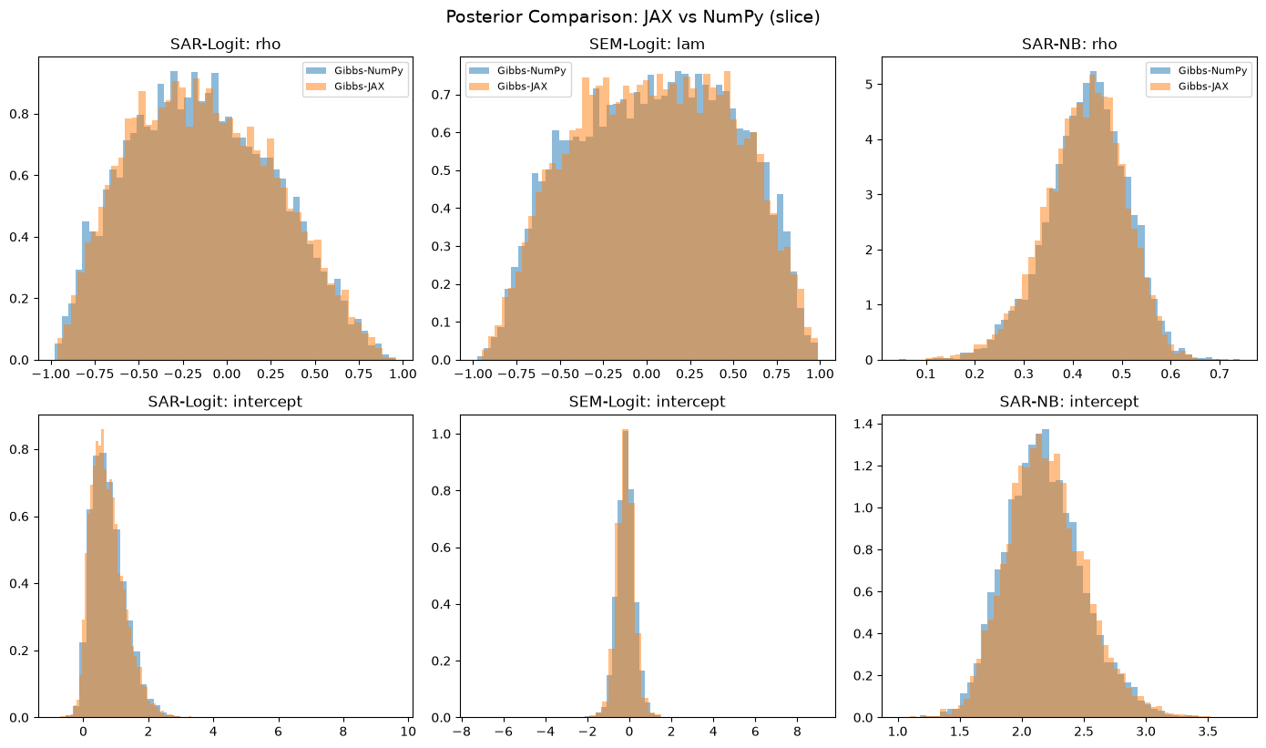
Compare posterior distributions across backends for each model. The JAX and NumPy posteriors should agree closely for well-identified parameters.

# Re-fit all models and store idatas for comparison plots
idatas = {}
for model_name, ModelClass, y, X in models_and_data:
    idatas[model_name] = {}
    for config_name, config in configs.items():
        model = ModelClass(y=y, X=X, W=W)
        try:
            idata = model.fit(**config)
            idatas[model_name][config_name] = idata
        except Exception:
            pass

# Plot comparison for each model
spatial_param_map = {"SAR-Logit": "rho", "SEM-Logit": "lam", "SAR-NB": "rho"}

fig, axes = plt.subplots(2, 3, figsize=(14, 8))

for col, model_name in enumerate(["SAR-Logit", "SEM-Logit", "SAR-NB"]):
    param = spatial_param_map[model_name]
    for row, param_name in enumerate([param, "beta"]):
        ax = axes[row, col]
        for config_name in configs:
            if config_name in idatas.get(model_name, {}):
                idata = idatas[model_name][config_name]
                if param_name == "beta":
                    # Plot intercept (first coefficient)
                    samples = idata.posterior["beta"].values[:, :, 0].flatten()
                else:
                    samples = idata.posterior[param_name].values.flatten()
                ax.hist(samples, bins=50, alpha=0.5, density=True, label=config_name)
        ax.set_title(
            f"{model_name}: {param_name if param_name != 'beta' else 'intercept'}"
        )
        if row == 0:
            ax.legend(fontsize=8)

plt.tight_layout()
plt.suptitle("Posterior Comparison: JAX vs NumPy (slice)", y=1.02, fontsize=14)
plt.show()

/home/runner/micromamba/envs/test/lib/python3.14/site-packages/neighbayes/samplers/negbin_reduced/__init__.py:85: UserWarning: SAR Negative Binomial models require large samples for reliable spatial parameter recovery. With n=49, posterior estimates of ρ and α may be severely attenuated. n ≥ 900 is recommended.
  return model._fit_gibbs(

../_images/55e5de89a3f7b877768c47e841d476c897e3c6765f4891f56beaf4ca1980c0f6.png

7. ESS per Second Comparison¶

Effective sample size per second measures sampling efficiency — higher is better. The JAX path’s full-JIT compilation eliminates Python dispatch overhead, and the Krylov basis provides cheap density evaluations for the NB ρ-slice.

# Compute ESS/sec for the spatial parameter
ess_per_sec = []
for model_name in ["SAR-Logit", "SEM-Logit", "SAR-NB"]:
    param = spatial_param_map[model_name]
    for config_name in configs:
        if config_name in idatas.get(model_name, {}):
            idata = idatas[model_name][config_name]
            ess = float(az.summary(idata, var_names=[param]).loc[param, "ess_bulk"])
            elapsed = [
                r["elapsed_s"]
                for r in results
                if r["label"] == f"{model_name}/{config_name}"
            ]
            t = elapsed[0] if elapsed else 1.0
            ess_per_sec.append(
                {
                    "Model": model_name,
                    "Sampler": config_name,
                    "ESS_bulk": int(ess),
                    "Time (s)": t,
                    "ESS/sec": round(ess / t, 1),
                }
            )

ess_df = pd.DataFrame(ess_per_sec)
if len(ess_df) > 0:
    pivot_ess = ess_df.pivot(index="Model", columns="Sampler", values="ESS/sec")
    if "Gibbs-NumPy" in pivot_ess.columns and "Gibbs-JAX" in pivot_ess.columns:
        pivot_ess["JAX ESS/sec ratio"] = (
            pivot_ess["Gibbs-JAX"] / pivot_ess["Gibbs-NumPy"]
        )
    print("ESS per second for spatial parameter (ρ/λ):")
    display(pivot_ess.round(1))
else:
    print("No ESS data available.")

ESS per second for spatial parameter (ρ/λ):

Sampler	Gibbs-JAX	Gibbs-NumPy	JAX ESS/sec ratio
Model
SAR-Logit	2392.9	597.4	4.0
SAR-NB	680.3	174.8	3.9
SEM-Logit	2131.5	248.5	8.6

8. Scaling: Effect of n on JAX vs NumPy Time¶

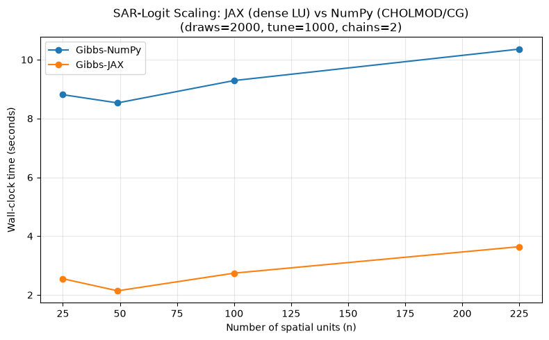
How does wall-clock time scale with the number of spatial units? The JAX path uses dense LU (O(n³)) while NumPy uses CHOLMOD/CG sparse solves — the crossover depends on sparsity and problem size.

SCALE_DRAWS = 2000
SCALE_TUNE = 1000
SCALE_CHAINS = 2
SIDES = [5, 7, 10, 15]  # n = 25, 49, 100, 225

scale_results = []

scale_configs = {
    "Gibbs-NumPy": dict(
        sampler="gibbs",
        gibbs_backend="numpy",
        n_jobs=-1,
        draws=SCALE_DRAWS,
        tune=SCALE_TUNE,
        chains=SCALE_CHAINS,
        random_seed=SEED,
        progressbar=False,
    ),
}
if HAS_JAX:
    scale_configs["Gibbs-JAX"] = dict(
        sampler="gibbs",
        gibbs_backend="jax",
        draws=SCALE_DRAWS,
        tune=SCALE_TUNE,
        chains=SCALE_CHAINS,
        random_seed=SEED,
        progressbar=False,
    )

for side in SIDES:
    n_s = side * side
    W_dense_s = make_rook_W(side)
    W_s = W_to_graph(W_dense_s)
    rng_s = np.random.default_rng(SEED)
    out_s = simulate_sar_logit(W=W_dense_s, rho=0.5, rng=rng_s)
    y_s, X_s = out_s["y"], out_s["X"]

    print(f"\nn = {n_s} (side={side})")
    for config_name, config in scale_configs.items():
        label = f"n={n_s}/{config_name}"
        model = SARLogit(y=y_s, X=X_s, W=W_s)
        try:
            result = profile_model(model, config, label)
            print(f"  {config_name}: {result['elapsed_s']:.1f}s")
            result["n"] = n_s
            result["sampler"] = config_name
            scale_results.append(result)
        except Exception as e:
            print(f"  {config_name}: FAILED ({e})")

print("\nScaling benchmark complete.")

n = 25 (side=5)
  Gibbs-NumPy: 8.8s
  Gibbs-JAX: 2.5s

n = 49 (side=7)
  Gibbs-NumPy: 8.5s
  Gibbs-JAX: 2.1s

n = 100 (side=10)
  Gibbs-NumPy: 9.3s
  Gibbs-JAX: 2.7s

n = 225 (side=15)
  Gibbs-NumPy: 10.4s
  Gibbs-JAX: 3.6s

Scaling benchmark complete.

# Plot scaling results
if scale_results:
    scale_df = pd.DataFrame(scale_results)
    fig, ax = plt.subplots(figsize=(8, 5))
    for sampler in scale_df["sampler"].unique():
        sub = scale_df[scale_df["sampler"] == sampler].sort_values("n")
        ax.plot(sub["n"], sub["elapsed_s"], marker="o", label=sampler)
    ax.set_xlabel("Number of spatial units (n)")
    ax.set_ylabel("Wall-clock time (seconds)")
    ax.set_title(
        f"SAR-Logit Scaling: JAX (dense LU) vs NumPy (CHOLMOD/CG)\n"
        f"(draws={SCALE_DRAWS}, tune={SCALE_TUNE}, chains={SCALE_CHAINS})"
    )
    ax.legend()
    ax.grid(True, alpha=0.3)
    plt.tight_layout()
    plt.show()
else:
    print("No scaling results to plot.")

../_images/4cf80f196be255f62c22d77a3f76a8061f82acd8e408c07af051887d5da31cb6.png

9. Summary¶

Both the NumPy and JAX Gibbs backends use slice sampling for the ρ/λ update. The key difference is the linear algebra backend:

NumPy (`gibbs_backend="numpy"`): CHOLMOD/CG sparse solves¶

Factorises \(A^T A = I - \rho(W+W^T) + \rho^2 W^T W\) via CHOLMOD (when available) or SuperLU.
Uses CG iterative solves when CHOLMOD is unavailable or n is large.
Exploits sparsity: O(nnz^{1.5}) for CHOLMOD, O(K·nnz) for CG.
Best for large, sparse W where the dense O(n³) cost is prohibitive.

JAX (`gibbs_backend="jax"`): sparse solves, JIT-compiled¶

Factorises \(A_\rho = I - \rho W\) once per sweep. The JAX path uses the sparse sparsax solve and never densifies \(W\); a dense jax.scipy.linalg.lu_factor fallback runs only when sparsax is unavailable, or on GPU.
Builds the Krylov basis with (m+1) lu_solve calls, then evaluates slice candidates via Horner — O(m·n·k) per candidate.
Full JIT compilation: the entire Gibbs step (including the Krylov build + slice sampling) is a single XLA kernel.
Best for small-to-medium problems (n ≤ ~2000 on CPU) where JIT eliminates Python dispatch overhead.

Why slice sampling everywhere?¶

MALA was tried for both logit and NB JAX paths but was significantly slower:

Logit: MALA requires jax.value_and_grad through jnp.linalg.solve, which traces through Cholesky+solve backward (~3× forward cost), called twice per step (current + proposed). This made JAX logit 3.6× slower than NumPy. Slice sampling avoids gradients entirely — each candidate needs only a forward density evaluation.
NB reduced form: Same autodiff bottleneck — jnp.linalg.solve backward pass is O(n³), making MALA 25× slower than NumPy. The Krylov basis provides cheap density evaluations for slice sampling.

Common features¶

Krylov basis (NB only): Both backends build \(V_j = A_\rho^{-1}(W V_{j-1})\) at the current ρ and evaluate U(ρ) via Horner for each slice candidate.
No logdet (NB reduced form): The reduced form’s β-marginalised ρ density does not include log|I−ρW| — it cancels when β is integrated out.
Intercept reparameterisation (NB): \(\delta_0 = \beta_0/(1-\rho)\) breaks the ρ–β₀ posterior correlation that causes ESS collapse at high ρ.