2 Geoprocessing

Spatial data comes in a rich variety of forms and corresponding file formats. At the beginning of most geocomputational workflows, one is typically reading these different formats and applying different forms of spatial data processing (or geoprocessing) methods to the data.

In this notebook we cover a subset of geoprocessing methods:

Reading & Writing geospatial data
Coordinate reference system transformations
Spatial joins
Spatial aggregations

Along the way we introduce the package geopandas which provides key spatial data processing functionality. The core data structure for spatial analysis in Python is the GeoDataFrame, which provides a tabular representation and stores geographic information as a special kind of attribute.

Code

import geopandas as gpd
import pandas as pd
from geosnap import DataStore
from geosnap import io as gio

datasets = DataStore()

OMP: Info #276: omp_set_nested routine deprecated, please use omp_set_max_active_levels instead.

Code

sea_ejscreen = gio.get_ejscreen(datasets, msa_fips="42660", years=2019)
sea_ejscreen = sea_ejscreen.to_crs(4326)  # convert to lat/long

We start by loading data from the The EPA’s Environmental Justic Screening Tool (EJSCREEN), which contains data on vulnerable populations, and spatial externalities that may have negative health consequences. The EPA processes these together into a composite “EJ” indicator that yields high values when vulnerable populations are exposed to high risks. The dataset also includes information for the national percentile ranking of each indicator for each blockgroup. The most useful data include the pure “risk” indicators listed below:

Variable	Description
DSLPM	Diesel particulate matter level in air
CANCER	Air toxics cancer risk
RESP	Air toxics respiratory hazard index
PTRAF	Traffic proximity and volume
PWDIS	Indicator for major direct dischargers to water
PNPL	Proximity to National Priorities List (NPL) sites
PRMP	Proximity to Risk Management Plan (RMP) facilities
PTSDF	Proximity to Treatment Storage and Disposal (TSDF) facilities
OZONE	Ozone level in air
PM25	PM2.5 level in air

Code

sea_ejscreen.head()

	geoid	ACSTOTPOP	ACSIPOVBAS	ACSEDUCBAS	ACSTOTHH	ACSTOTHU	MINORPOP	MINORPCT	LOWINCOME	LOWINCPCT	...	T_PM25_P2	T_PM25_P6	AREALAND	AREAWATER	Shape_Length	Shape_Area	geometry	year
0	530330001001	1265	1235	1095	608	608	155	0.122530	136	0.110121	...	7%ile	12%ile	892826.0	904304.0	8633.745188	3.969193e+06	MULTIPOLYGON (((-122.28977 47.73374, -122.2884...	2019
1	530330001002	1534	1527	1210	758	871	765	0.498696	558	0.365422	...	54%ile	54%ile	288190.0	0.0	3940.705233	6.365748e+05	MULTIPOLYGON (((-122.29654 47.73015, -122.2952...	2019
2	530330001003	1817	1817	1263	724	738	731	0.402312	543	0.298844	...	44%ile	28%ile	370737.0	0.0	3878.874929	8.187073e+05	MULTIPOLYGON (((-122.29321 47.72291, -122.2929...	2019
3	530330001004	2270	2270	1332	1052	1134	1622	0.714537	1283	0.565198	...	71%ile	67%ile	126662.0	0.0	2128.066919	2.798096e+05	MULTIPOLYGON (((-122.29656 47.73198, -122.2965...	2019
4	530330001005	1077	1077	808	637	679	393	0.364903	314	0.291551	...	41%ile	41%ile	230515.0	0.0	3376.927631	5.090533e+05	MULTIPOLYGON (((-122.29642 47.72651, -122.2946...	2019

5 rows × 368 columns

Code

sea_ejscreen.shape

(2483, 368)

This dataset has 2,483 observations (rows) and 368 attributes (columns)

Code

sea_ejscreen.columns

Index(['geoid', 'ACSTOTPOP', 'ACSIPOVBAS', 'ACSEDUCBAS', 'ACSTOTHH',
       'ACSTOTHU', 'MINORPOP', 'MINORPCT', 'LOWINCOME', 'LOWINCPCT',
       ...
       'T_PM25_P2', 'T_PM25_P6', 'AREALAND', 'AREAWATER', 'NPL_CNT',
       'TSDF_CNT', 'Shape_Length', 'Shape_Area', 'geometry', 'year'],
      dtype='object', length=368)

The sea_ejscreen GeoDataFrame is a special kind of pandas DataFrame that stores information about the geometric information associated with each record in the dataset. As such, any pandas operation will work as normal; to demonstrate, lets rename the ‘ACSTOTPOP’ column to ‘total_population’. Note that we need to re-save the dataframe back into a variable to store the change.

Code

sea_ejscreen.columns[1]

'ACSTOTPOP'

Code

sea_ejscreen = sea_ejscreen.rename(columns={"ACSTOTPOP": "total_population"})

Code

sea_ejscreen.columns[1]

'total_population'

See the second column (remember Python indexing begins at zero!) now has the updated name

Two important pieces of information distinguish a GeoDataFrame from a simple aspatial DataFrame: a ‘geometry’ column that defines the shape and of each feature, and a Coordinate Reference System (CRS) that stores metadata about how the shape is encoded.

Code

sea_ejscreen.geometry

0       MULTIPOLYGON (((-122.28977 47.73374, -122.2884...
1       MULTIPOLYGON (((-122.29654 47.73015, -122.2952...
2       MULTIPOLYGON (((-122.29321 47.72291, -122.2929...
3       MULTIPOLYGON (((-122.29656 47.73198, -122.2965...
4       MULTIPOLYGON (((-122.29642 47.72651, -122.2946...
                              ...                        
2478    MULTIPOLYGON (((-122.31386 48.07283, -122.3130...
2479    MULTIPOLYGON (((-122.32737 48.12333, -122.3256...
2480    MULTIPOLYGON (((-122.36870 48.12337, -122.3632...
2481    MULTIPOLYGON (((-122.44294 47.79322, -122.4429...
2482    MULTIPOLYGON (((-122.45861 48.29771, -122.4520...
Name: geometry, Length: 2483, dtype: geometry

Since the Seattle blockgroups are polygons, naturally they are represented as a shapely Polygon (or MultiPolygon, meaning there are multiple shapes that combine to create a single blockgroup) object. This means, essentially, that each polygon is represented as a set of coordinates that define the polygon border. The units of those coordinates are stored in the GeoDataFrame’s Coordinate Reference System attribute crs

Code

sea_ejscreen.crs

<Geographic 2D CRS: EPSG:4326>
Name: WGS 84
Axis Info [ellipsoidal]:
- Lat[north]: Geodetic latitude (degree)
- Lon[east]: Geodetic longitude (degree)
Area of Use:
- name: World.
- bounds: (-180.0, -90.0, 180.0, 90.0)
Datum: World Geodetic System 1984 ensemble
- Ellipsoid: WGS 84
- Prime Meridian: Greenwich

In this case, the blockgroups stored in Latitude/Longitude using the well-known WGS84 datum. Latitude/Longitude is called a ‘geographic coordinate system’ because the coordinates refer to locations on a spheroid, and the data have not been projected onto a flat plane.

Code

sea_ejscreen.crs.is_projected

False

Code

sea_ejscreen.crs.is_geographic

True

Naturally, the CRS defined on the GeoDataFrame governs the behavior of any spatial operation performed against the dataset, like computing the area of each polygon, the area of intersection with another dataset, or the distance between observations

Code

sea_ejscreen.area

/var/folders/79/cknfb1sx2pv16rztkpg6wzlw0000gn/T/ipykernel_86094/554462416.py:1: UserWarning: Geometry is in a geographic CRS. Results from 'area' are likely incorrect. Use 'GeoSeries.to_crs()' to re-project geometries to a projected CRS before this operation.

  sea_ejscreen.area

0       0.000215
1       0.000035
2       0.000044
3       0.000015
4       0.000028
          ...   
2478    0.000457
2479    0.002580
2480    0.002256
2481    0.021275
2482    0.001603
Length: 2483, dtype: float64

Note that we get a warning from GeoPandas when trying to compute the are of a polygon stored in a geographic CRS. But we can estimate an appropriate Universal Transverse Mercator (UTM) Zone for the center of the Seattle Metro dataset, then reproject the blockgroups into that system, and recompute the area.

Code

# get the UTM zone for Chicago
utm_crs = sea_ejscreen.estimate_utm_crs()
utm_crs

<Projected CRS: EPSG:32610>
Name: WGS 84 / UTM zone 10N
Axis Info [cartesian]:
- E[east]: Easting (metre)
- N[north]: Northing (metre)
Area of Use:
- name: Between 126°W and 120°W, northern hemisphere between equator and 84°N, onshore and offshore. Canada - British Columbia (BC); Northwest Territories (NWT); Nunavut; Yukon. United States (USA) - Alaska (AK).
- bounds: (-126.0, 0.0, -120.0, 84.0)
Coordinate Operation:
- name: UTM zone 10N
- method: Transverse Mercator
Datum: World Geodetic System 1984 ensemble
- Ellipsoid: WGS 84
- Prime Meridian: Greenwich

Seattle falls inside UTM Zone 10 North (apparently), and since UTM is measured in meters, the second area calculation shows the (correct) area of each blockgroup as square kilometers.

Code

# reproject into UTM and convert area in square meters to square kilometers
sea_ejscreen.to_crs(utm_crs).area / 1e6

0         1.795820
1         0.287980
2         0.370467
3         0.126570
4         0.230347
           ...    
2478      3.781797
2479     21.355873
2480     18.671198
2481    176.442839
2482     13.218388
Length: 2483, dtype: float64

One other difference between a DataFrame and a GeoDataFrame is the plot method has been overloaded to generate a quick map

Code

sea_ejscreen.plot()

2.1 Reading and Writing Data

2.1.1 Legacy File Formats

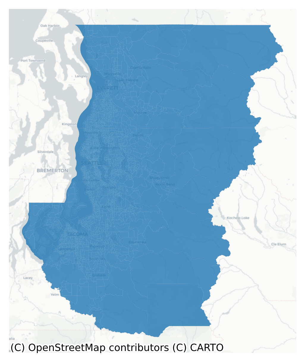
Inevitably, many analysts will encounter geospatial data stored in a variety of formats, such as GeoJSON, Shapefile, or GeoPackage. I recommend you avoid these formats whenever possible, and instead adopt the geoparquet file standard, recently adopted by the Open Geospatial Consortium (OGC),

Code

# shapefile
sea_ejscreen.to_file("sea_ejscreen.shp")

# geopackage
sea_ejscreen.to_file("sea_ejscreen.gpkg")

# geoJSON
sea_ejscreen.to_file("sea_ejscreen.geojson")

/var/folders/79/cknfb1sx2pv16rztkpg6wzlw0000gn/T/ipykernel_86094/2797242796.py:2: UserWarning: Column names longer than 10 characters will be truncated when saved to ESRI Shapefile.
  sea_ejscreen.to_file("sea_ejscreen.shp")

GeoPandas is smart enough to infer the file type from the extension provided in the output file name (but this can be overridden with the driver argument). Notice how long this cell takes to execute!

And you can read a GeoDataFrame into memory from a file on disk similarly

Code

# re-read the exported data into a new variable
sea_ejscreen_shp = gpd.read_file("sea_ejscreen.shp")

Remember, though, that because of the inherent properties of these file types, sometimes “round-tripping” (i.e. writing a dataset to disk then re-reading it into memory) can lose information! For example writing to a shapefile will truncate any column names longer than 10 characters, and writing to GeoJSON will lose any coordinate system metadata…

Code

sea_ejscreen_shp.columns[1]

'total_popu'

Note that in sea_ejscreen_shp the ‘total_population’ column has been truncated back to ‘total_popu’

2.1.2 Modern File Formats

Code

import os

sea_ejscreen.to_parquet("sea_ejscreen.parquet")

Code

for ext in ["parquet", "gpkg", "geojson"]:
    size = os.path.getsize(f"sea_ejscreen.{ext}")
    print(f"{ext} is {round(size / 1e6, 2)} MB")

parquet is 10.28 MB
gpkg is 15.46 MB
geojson is 43.53 MB

For this dataset, the geopackage storage is 1.5x the size the parquet file, and the GeoJSON file is more than 4x(!) the file size. The tradeoff is that GeoJSON is a simple text file that can be opened and edited with any editor; the geopackage is a special kind of SQLite database accessible by sqlite editor, and the parquet file is a compressed binary that needs an open-source driver to be decoded

2.2 Geospatial Operations

Geopandas can carry out all standard GIS operations using methods implemented on a GeoDataFrame, for example

clip: “cut” the extent of one dataset using the boundaries of another
dissolve: aggregate geometries using a common value from an attribute (e.g. remove interior boundaries from larger container polygons, e.g. counties within a state)
simplify: remove vertices from the input geometries
buffer: extend the boundaries of input geometries by a fixed distance (always returns polygons)
centroid: compute the geometric center of input geometries (always returns points)
convex/concave hull: compute the most efficient convex/convave polygon that contains vertices from all input geometries

By combining these operations along with spatial predicates, we can create queries based on the topological relationships between two sets of geographic units, which is often critical for creating variables of interest.

To demonstrate, we will first collect data from OpenStreetMap (OSM), specifically highways in the Seattle metro. In OSM parlance, this means we’re querying for “highways” with the “motorway” tag (which means “the highest-performance roads within a territory. It should be used only on roads with control of access, or selected roads with limited access depending on the local context and prevailing convention. Those roads are generally referred to as motorways, freeways or expressways in English.”)

Code

import osmnx as ox

Code

highways = ox.features_from_polygon(
    sea_ejscreen.unary_union, tags={"highway": "motorway"}
)

This returns a new GeoDataFrame storing each highway as a line feature.

Code

highways.head()

		highway	geometry	ref	nodes	bus:lanes	hgv	hov	hov:lanes	hov:minimum	lanes	...	motorcycle:lanes:conditional	sidewalk	hov:lanes:backward	hov:lanes:forward	hazmat	start_date	sidewalk:left	sidewalk:right	bridge:movable	wikidata
element_type	osmid
way	5155365	motorway	LINESTRING (-122.20833 47.46902, -122.20868 47...	I 405	[5123200942, 6682413518]	designated\|\|	designated	yes	designated\|\|	2	3	...	NaN	NaN	NaN	NaN	NaN	NaN	NaN	NaN	NaN	NaN
	5155547	motorway	LINESTRING (-122.20086 47.48021, -122.20123 47...	I 405	[677281419, 35830168, 35830169, 35830170, 1006...	designated\|\|\|	designated	yes	designated\|\|\|	2	4	...	NaN	NaN	NaN	NaN	NaN	NaN	NaN	NaN	NaN	NaN
	6503478	motorway	LINESTRING (-122.12159 47.35782, -122.12202 47...	SR 18	[53203320, 53246032, 53246031, 53246030, 25722...	NaN	NaN	NaN	NaN	NaN	2	...	NaN	NaN	NaN	NaN	NaN	NaN	NaN	NaN	NaN	NaN
	6503481	motorway	LINESTRING (-121.97495 47.43581, -121.97525 47...	SR 18	[53245950, 257175427, 53244286, 257175814]	NaN	NaN	NaN	NaN	NaN	2	...	NaN	NaN	NaN	NaN	NaN	NaN	NaN	NaN	NaN	NaN
	8562291	motorway	LINESTRING (-122.13853 47.34822, -122.13926 47...	SR 18	[53241943, 53245949]	NaN	NaN	NaN	NaN	NaN	2	...	NaN	NaN	NaN	NaN	NaN	NaN	NaN	NaN	NaN	NaN

5 rows × 105 columns

Code

highways.plot()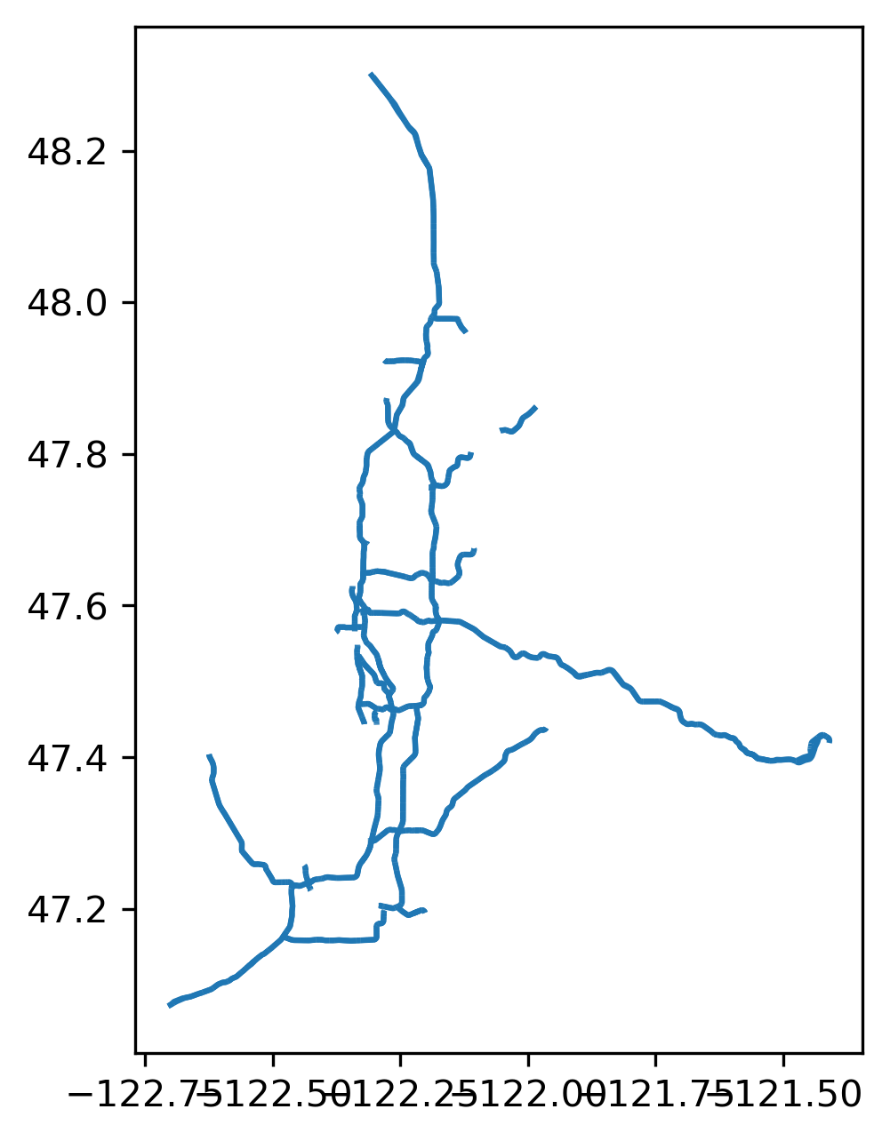

Notice in the call to features_from_polygon above, we used the unary_union operator on the Seattle tracts dataframe. This effectively combines all the tracts into a single polygon so we are querying anything that intersects any tract, rather than querying intersections with each tract individually. We can do the same thing on the highway GeoDataFrame to see the effect

Code

# note in geopandas >=1.0 this is `highways.union_all()`

hw_union = highways.unary_union

Code

hw_union

Now hw_union is a single shapely.Polygon with no attribute information

Code

gpd.GeoDataFrame(geometry=[hw_union], crs=4326).explore(tiles='CartoDB Positron')

Make this Notebook Trusted to load map: File -> Trust Notebook

(Why isn’t that tiny section of State Highway 522 connected up in the Northeast? I have no idea.)

2.3 Integrating Spatial Datasets

Let’s assume the role of a public health epidemiologist who is interested in equity issues surrounding exposure to highways and automobile emissions. We may be interested in who lives near the highway and whether the population nearby experiences a heightened exposure to toxic emissions.

2.3.1 Select by Location

One simple question would be, which tracts have a highway run through them? We can formalize that by asking which tracts intersect the highway system.

Code

highway_blockgroups = sea_ejscreen[sea_ejscreen.intersects(hw_union)]
highway_blockgroups.plot()

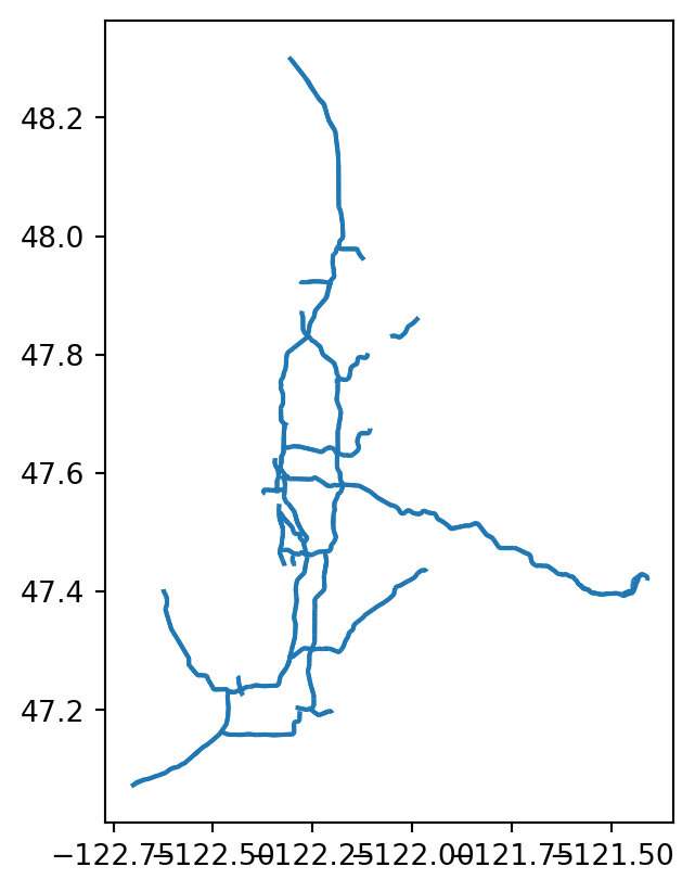
A more complicated question is, which tracts are within 1.5km of a road? This is ‘complicated’ because it forces us to formalize an ill-defined relationship: the distance between a polygon and the nearest point on a line. What does it mean for the polygon to be ‘within’ 1.5km? Does that mean the whole tract? most of it? any part of it?

If we can define a most suitable distance measure, the technical selection is easy to execute using an intermediate geometry.

Code

road_buffer = highways.to_crs(highways.estimate_utm_crs()).buffer(1500)

Code

gpd.GeoDataFrame(geometry=[road_buffer.unary_union], crs=road_buffer.crs).explore(tiles='CartoDB Positron')

Make this Notebook Trusted to load map: File -> Trust Notebook

Code

sea_ejscreen.crs

<Geographic 2D CRS: EPSG:4326>
Name: WGS 84
Axis Info [ellipsoidal]:
- Lat[north]: Geodetic latitude (degree)
- Lon[east]: Geodetic longitude (degree)
Area of Use:
- name: World.
- bounds: (-180.0, -90.0, 180.0, 90.0)
Datum: World Geodetic System 1984 ensemble
- Ellipsoid: WGS 84
- Prime Meridian: Greenwich

Code

sea_ejscreen[sea_ejscreen.intersects(road_buffer.unary_union)]

	geoid	total_population	ACSIPOVBAS	ACSEDUCBAS	ACSTOTHH	ACSTOTHU	MINORPOP	MINORPCT	LOWINCOME	LOWINCPCT	...	T_PM25_P2	T_PM25_P6	AREALAND	AREAWATER	NPL_CNT	TSDF_CNT	Shape_Length	Shape_Area	geometry	year

0 rows × 368 columns

This gives us back nothing… There is no intersection because the EJSCREEN data is still stored in Lat/Long, but we reprojected the road buffer into UTM

Code

sea_ejscreen = sea_ejscreen.to_crs(road_buffer.crs)

By selecting the tracts that intersect with the interstate buffer, we are codifying the tracts as ‘near the highway’ if any portion of a tract is within 1.5km. This can be an awkard choice when polygons are irregularly shaped or heteogeneously sized (Census tracts are both). This means large tracts get included as ‘near’, even when a small portion of the polygon is within the 1.5km threshold (like the tract on the far Eastern edge).

Code

sea_ejscreen[sea_ejscreen.intersects(road_buffer.unary_union)].plot()

Alternatively, we might ask, which tracts have their center within 1.5km of a highway? Or more formally, which tracts have their centroids intersect with the 1500m buffer.

Code

sea_ejscreen[sea_ejscreen.centroid.intersects(road_buffer.unary_union)].plot()

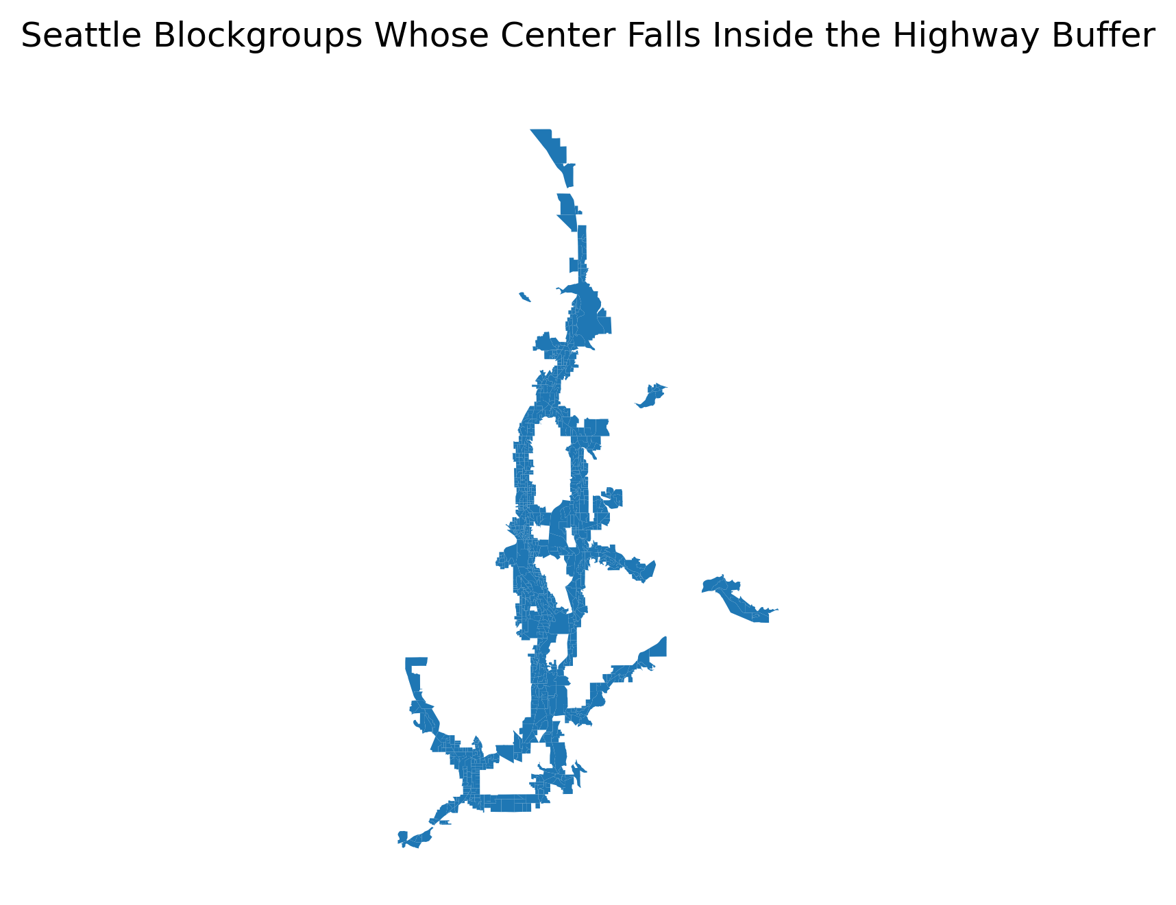
If we are happy with that definition of proximity, we can use the spatial selection to create and update a new attribute on the dataframe. Here, we will select the tracts whose centroids are within the threshold distance, then create a new column called “highway_buffer”, set to “inside” (using the indices of the spatial selection to define which rows are being set).

Code

# get the dataframe index of the tracts intersecting the buffer

inside_idx = sea_ejscreen[
    sea_ejscreen.centroid.intersects(road_buffer.unary_union)
].index

Code

# set the 'highway_buffer' attribute to 'inside' for the indices within
sea_ejscreen.loc[inside_idx, "highway_buffer"] = "inside"

# fill all NaN values in the column with 'outside'
sea_ejscreen["highway_buffer"] = sea_ejscreen["highway_buffer"].fillna("outside").astype('category')

Now ‘highway_buffer’ is a binary variable defining whether a tract is “near” a highway or not. We could have set these values to one and zero, but setting them as a categorical variable means that the geopandas plot method uses a different kind of coloring scheme that matches the data more appropriately.

Code

sea_ejscreen[['highway_buffer', 'geometry']].explore("highway_buffer", legend=True, tiles='CartoDB Positron')

Make this Notebook Trusted to load map: File -> Trust Notebook

Then, we can use this spatial distinction as a grouping variable to look at average values inside versus outside the threshold zone.

Code

sea_ejscreen.groupby("highway_buffer")[["PM25", "DSLPM", "MINORPCT"]].mean()

/var/folders/79/cknfb1sx2pv16rztkpg6wzlw0000gn/T/ipykernel_86094/860608503.py:1: FutureWarning: The default of observed=False is deprecated and will be changed to True in a future version of pandas. Pass observed=False to retain current behavior or observed=True to adopt the future default and silence this warning.
  sea_ejscreen.groupby("highway_buffer")[["PM25", "DSLPM", "MINORPCT"]].mean()

	PM25	DSLPM	MINORPCT
highway_buffer
inside	6.298818	1.043487	0.404843
outside	6.061902	0.723160	0.283832

On average, both PM2.5 and Disel Particulate Matter levels are higher for tracts located within 1.5km of an OSM ‘motorway’ (what we think is probably an interstate highway). The share of residents identifying as a racial or ethnic miority is also 12% higher on average.

2.3.2 Spatial Join

In the example above, we use only the geometric relationship between observations to make selections from one dataset. In other cases, we need to attach attribute data from one dataset to the other using spatial relationships. For example we might want to count the number of health clinics that fall inside each census tract. This actually entails two operations: attaching census tract identifiers to each clinic, then aggregating by tract identifier and counting all clinics within

Once again we will query OSM, this time looking for an amenity with the ‘clinic’ tag

Code

clinics = ox.features_from_polygon(
    sea_ejscreen.to_crs(4326).unary_union, tags={"amenity": "clinic"}
)
clinics = clinics.reset_index().set_index("osmid")

Code

clinics.head()

	element_type	amenity	healthcare	name	geometry	brand	brand:wikidata	healthcare:counselling	operator	operator:wikidata	...	official_name	short_name	social_facility	ele	ref	building:material	waste_disposal	wikidata	owner	layer
osmid
4774229656	node	clinic	clinic	Indigo Urgent Care	POINT (-122.21004 47.10002)	NaN	NaN	NaN	NaN	NaN	...	NaN	NaN	NaN	NaN	NaN	NaN	NaN	NaN	NaN	NaN
4881851935	node	clinic	clinic	Medical Center of Orting	POINT (-122.20330 47.09741)	NaN	NaN	NaN	NaN	NaN	...	NaN	NaN	NaN	NaN	NaN	NaN	NaN	NaN	NaN	NaN
4214385093	node	clinic	counselling	Planned Parenthood	POINT (-122.20496 47.38755)	Planned Parenthood	Q2553262	antenatal;sexual	Planned Parenthood	Q2553262	...	NaN	NaN	NaN	NaN	NaN	NaN	NaN	NaN	NaN	NaN
4461362475	node	clinic	clinic	Indigo Urgent Care	POINT (-122.11924 47.35842)	NaN	NaN	NaN	NaN	NaN	...	NaN	NaN	NaN	NaN	NaN	NaN	NaN	NaN	NaN	NaN
4461363953	node	clinic	clinic	Valley Medical Center - Lake Sawyer Clinic	POINT (-122.05587 47.35710)	NaN	NaN	NaN	NaN	NaN	...	NaN	NaN	NaN	NaN	NaN	NaN	NaN	NaN	NaN	NaN

5 rows × 112 columns

The clinics dataset now has manuy types of clinics, and also has a mixed geometry type; some clinics are stored as polygons (where the building footprint has been digitized) whereas others are simply stored as points. Lets filter the dataset to include only those defined as clinic (e.g. not counseling) and only points (not polygons)

Code

clinics = clinics[(clinics.healthcare == "clinic") & (clinics.element_type == "node")]

Code

clinics.explore(tiles='CartoDB Positron', tooltip=['name', 'healthcare'])

Make this Notebook Trusted to load map: File -> Trust Notebook

Code

clinics = clinics.to_crs(sea_ejscreen.crs)

Code

clinics_geoid = clinics.sjoin(sea_ejscreen[["geoid", "geometry"]])

Code

clinics_geoid.head()

	element_type	amenity	healthcare	name	geometry	brand	brand:wikidata	healthcare:counselling	operator	operator:wikidata	...	social_facility	ele	ref	building:material	waste_disposal	wikidata	owner	layer	index_right	geoid
osmid
4774229656	node	clinic	clinic	Indigo Urgent Care	POINT (559944.778 5216582.316)	NaN	NaN	NaN	NaN	NaN	...	NaN	NaN	NaN	NaN	NaN	NaN	NaN	NaN	1631	530530704033
4881851935	node	clinic	clinic	Medical Center of Orting	POINT (560459.307 5216297.284)	NaN	NaN	NaN	NaN	NaN	...	NaN	NaN	NaN	NaN	NaN	NaN	NaN	NaN	1630	530530704032
4461362475	node	clinic	clinic	Indigo Urgent Care	POINT (566511.299 5245370.976)	NaN	NaN	NaN	NaN	NaN	...	NaN	NaN	NaN	NaN	NaN	NaN	NaN	NaN	1226	530330317062
4461363953	node	clinic	clinic	Valley Medical Center - Lake Sawyer Clinic	POINT (571297.956 5245281.151)	NaN	NaN	NaN	NaN	NaN	...	NaN	NaN	NaN	NaN	NaN	NaN	NaN	NaN	1265	530330320062
4556359114	node	clinic	clinic	Allcare Medical Clinic	POINT (560125.882 5259322.896)	NaN	NaN	NaN	NaN	NaN	...	NaN	NaN	NaN	NaN	NaN	NaN	NaN	NaN	788	530330253013

5 rows × 114 columns

Now we want to count clinics in each geoid. Since we know osmid uniquely identifies each clinic, we can reset the index, then groupby the ‘geoid’ variable, counting the unique ’osmid’s in each one

Code

clinic_count = clinics_geoid.reset_index().groupby("geoid").count()["osmid"]

Code

clinic_count

geoid
530330001003    1
530330002002    1
530330006004    2
530330012004    1
530330013003    1
               ..
530610519252    1
530610527072    1
530610535093    1
530610538023    1
530610538024    1
Name: osmid, Length: 176, dtype: int64

clinic_count is now a pandas series where the index refers to the census tract of interest and the value corresponds to the number of clinics that fall inside.

Code

sea_ejscreen = sea_ejscreen.merge(
    clinic_count.rename("clinic_count"), left_on="geoid", right_index=True, how="left"
)

Code

sea_ejscreen.clinic_count

0       NaN
1       NaN
2       1.0
3       NaN
4       NaN
       ... 
2478    NaN
2479    NaN
2480    NaN
2481    NaN
2482    NaN
Name: clinic_count, Length: 2483, dtype: float64

Now the sea_ejscreen GeoDataFrame has a new column called ‘clinic_count’ that holds the number of clinics inside. Since we know that NaN (Not a number) refers to zero in this case, we can go ahead and fill the missing data.

Code

sea_ejscreen["clinic_count"] = sea_ejscreen["clinic_count"].fillna(0)

Code

sea_ejscreen[['clinic_count', 'geometry']].explore(
    "clinic_count", scheme='fisher_jenks', cmap='Reds', tiles='CartoDB Positron'
)

Make this Notebook Trusted to load map: File -> Trust Notebook

:::