30  Hedonic Models in Space

Code
import requests

import contextily as ctx
import geopandas as gpd
import pandas as pd
import numpy as np
import esda
import matplotlib.pyplot as plt
import seaborn as sns
import statsmodels.formula.api as smf

from formulaic import Formula
from geosnap import DataStore
from geosnap.io import get_acs, get_lodes, get_network_from_gdf
from libpysal.graph import Graph
from scipy.stats import zscore
from splot import esda as esdplt
from spreg import GMM_Error, GM_Lag, OLS, spsearch

%load_ext watermark
%watermark -a 'eli knaap' -iv
The watermark extension is already loaded. To reload it, use:
  %reload_ext watermark
Author: eli knaap

pandas     : 2.2.3
geopandas  : 1.0.1
formulaic  : 1.1.1
matplotlib : 3.10.0
esda       : 2.7.0
statsmodels: 0.14.4
requests   : 2.32.3
geosnap    : 0.15.3.dev3+g3fa22c0.d20250409
scipy      : 1.15.2
splot      : 1.1.7
seaborn    : 0.13.2
contextily : 1.6.2
spreg      : 1.9.dev28+g0b017db
libpysal   : 4.13.0
numpy      : 1.26.4

In the last chapter, several commonly-used model specifications were defined, but the choice among them depends on the research question. Naturally, if spillover effects are of substantive interest, then it is necessary to choose a model that includes (at least) \(\rho WY\) or \(\theta WX\), but beyond that, the choice is more complex. The literature basically offers two different strategies; Anselin & Rey (2014) argue that a “bottom-up” strategy is most effective, where we begin with simple models (e.g., OLS), then conduct spatial diagnostic tests to decide whether more complex specifications are necessary. LeSage (2014) and LeSage & Pace (2014) argue for a “top-down” strategy where we begin with a ‘fully specified’ conceptual model.

LeSage (2014, p. 19) goes so far as to say that “there are only two model specifications worth considering for applied work.” When there are theoretical reasons to consider global spillover processes (such as home prices in a hedonic model), then the SDM model is appropriate. In other cases that consider only local spillover effects, the SDEM specification will provide unbiased estimates of all parameters. Their logic (to always prefer the Durbin specifications) is simple: the inclusion of the \(\theta WX\) term ensures that if there is an exogenous spillover process, then it will be measured accurately with only a small efficiency penalty, but omitting the term would lead to bias. The distinction between the SDM versus the SDEM, however, is largely a theoretical choice for a given research question rather than an empirical matter. As LeSage & Pace (2014, p. 1551) describe:

“Global spillovers arise when changes in a characteristic of one region impact outcomes in more than just immediately neighboring regions. Global impacts fall on neighbors to the neighbors, neighbors to the neighbors to the neighbors, and so on… Local spillovers represent a situation where the impacts fall only on nearby or immediate neighbors, dying out before they impact regions that are neighbors to the neighbors… feedback effects arise in the case of global spillovers, but not in the case of local spillovers.”

It follows “that practitioners cannot simply estimate an SDM and SDEM model and draw meaningful conclusions about the correct model specification from point estimates of \(\rho\) or \(\lambda\)… the SDM specification implies global spatial spillovers, while the SDEM is consistent with local spillovers. These have very different policy implications in applied work” (LeSage, 2014, p. 22), because indirect (and total) effects will be underestimated in the case when SDM model is appropriate but the SDEM model is fit because SDEM does not include feedback effects.1

Different specifications imply different DGPs and reflect what you want to study.

The SAR and SDM models which contain the spatially-lagged dependent variable \(\rho Wy\) specify global spillovers; the SLX, SDM, and SDEM models which contain the \(\theta WX\) term specify local spillovers (SDM specifies both). The difference between global and local spillovers pertains to the ways that effects propagate through the system and the ways that model coefficients may be interpreted (Juhl, 2021); SAR assumes explicit spillover processes, whereas SEM assumes spatially correlated omitted variables. You should have theory guiding which specification you want to use, even though most applied work uses a fit-based model selection approach. As described in preceding sections, the difference between the different types of spillovers is a critical distinction for applied work and policy analysis because we generally need to consider marginal effects, which means computing direct and indirect effects for models including a spatial lag. In the examples below, we examine how to fit and compare diagnostics for these different models using the spreg package (Anselin & Rey, 2014; Rey et al., 2021; Rey & Anselin, 2010).

30.1 Data Preparation

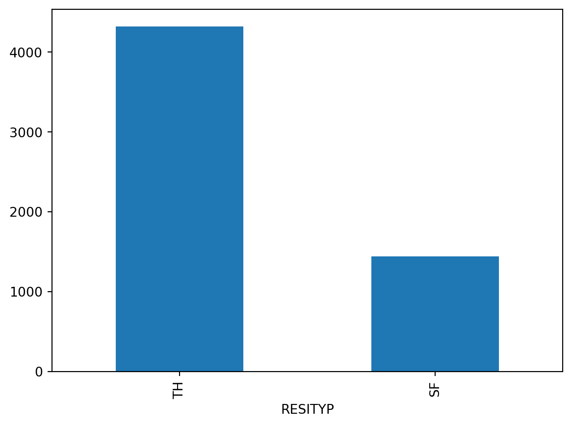
Since we are collecting raw parcel data, we will need to do a bit of cleanup and preparation before beginning model construction. The state of Maryland makes available a great set of parcel-level data called PropertyView, which include point and polygon datasets including attributes from the tax assessor’s’ office (e.g. size and sales price of the property, etc.). They also provide sales listings broken down by quarter or aggregated by year, and this is the dataset we use for the model. We will also attach these parcel points to the attributes of the blockgroup they fall inside.

Code
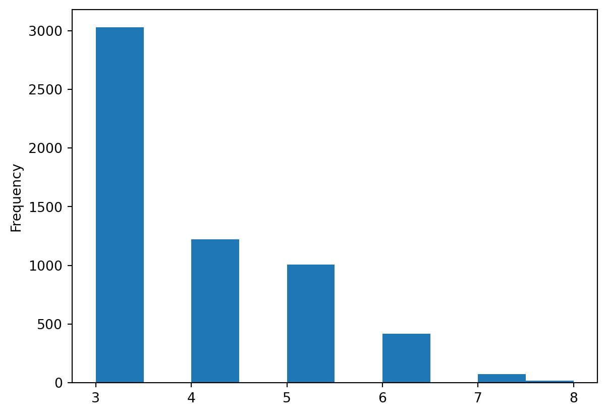
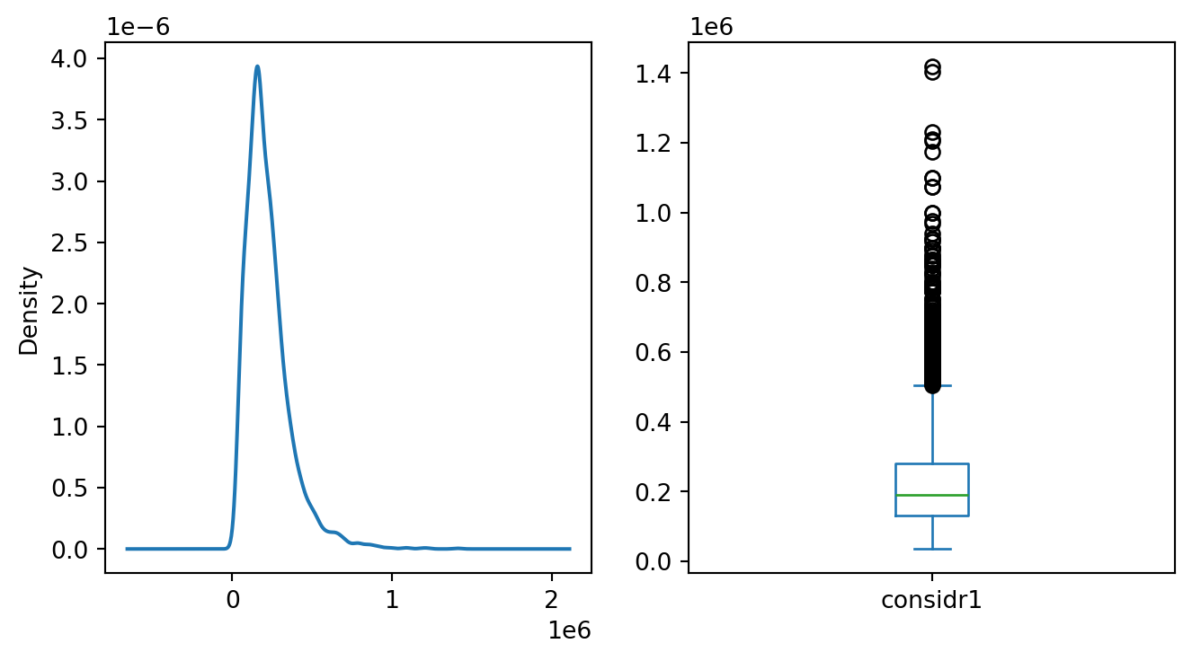
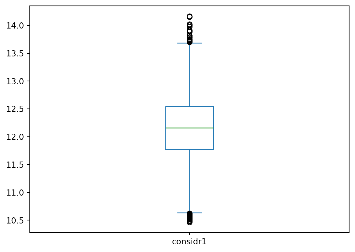
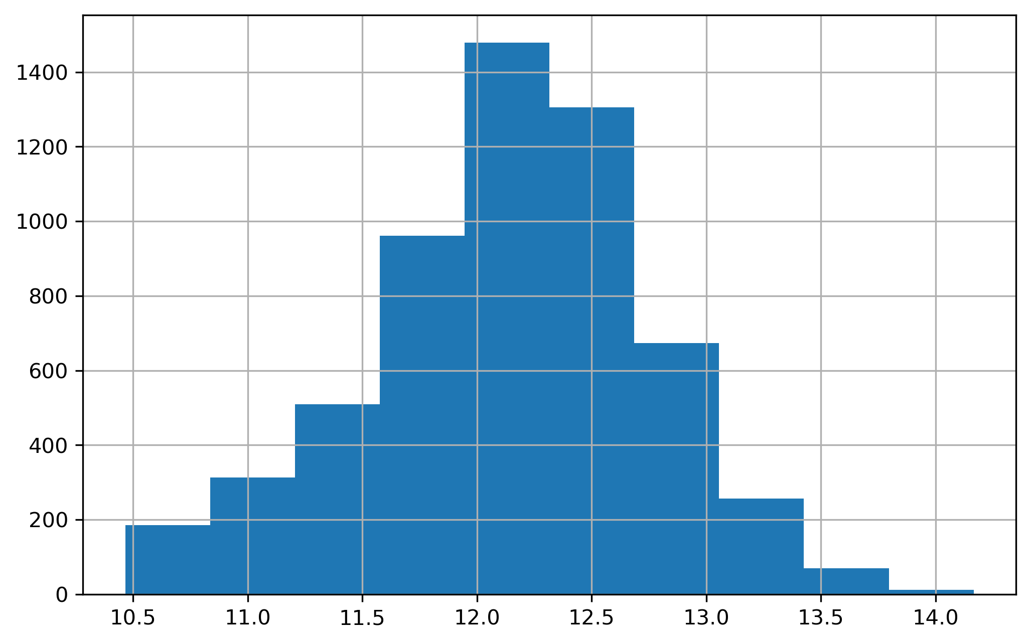
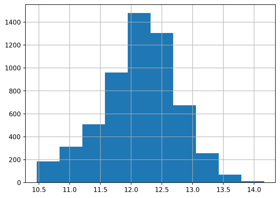
np.set_printoptions(suppress=True)  # prevent scientific format
datasets = DataStore()
balt_acs = get_acs(datasets, county_fips="24510", years=2019)
balt_lodes = get_lodes(datasets, county_fips="24510", years=2019)

# compute access variables
balt_net = get_network_from_gdf(balt_acs)
balt_lodes["node_ids"] = balt_net.get_node_ids(
    balt_lodes.centroid.x, balt_lodes.centroid.y
)
balt_net.set(balt_lodes["node_ids"], balt_lodes["total_employees"].values, name="jobs")
access = balt_net.aggregate(2000, name="jobs", decay="exp")

# download PropertyView data and read as a geodataframe
headers = {"user-agent": "Wget/1.16 (linux-gnu)"}
zfilename = "BACIparcels0225.zip"
# download the zip file onto the local disk
z = requests.get(
    "https://www.dropbox.com/scl/fi/xub9kdq5eug6pcsiib0bf/BACIparcels0225.zip?rlkey=f5zwjp7uyl7xpzkmep9o92aec&st=9vc03ft5&dl=0",
    stream=True,
    headers=headers,
)
with open(f"./{zfilename}", "wb") as f:
    f.write(z.content)
gdf = gpd.read_file("./BACIparcels0225.zip", layer="BACIMDPV")
gdf = gdf.set_index("ACCTID")


zfilename = "Statewide-Res-Sales-CY2018.zip"
# get the 2018 Sales data to join to parcel points
z = requests.get(
    "https://www.dropbox.com/s/sstsedw9bhtlhyw/Statewide-Res-Sales-CY2018.zip",
    stream=True,
    headers=headers,
)
with open(f"./{zfilename}", "wb") as f:
    f.write(z.content)

sales = gpd.read_file("./Statewide-Res-Sales-CY2018.zip")
sales = sales.set_index("acctid")
# keep only sales from 2018, drop duplicate geom column
# CRS in this file is epsg:26985 (meters)
balt_sales = sales.join(gdf.drop(columns=["geometry"]), how="inner")

# attach job access data
balt_sales["node_ids"] = balt_net.get_node_ids(
    balt_sales.to_crs(4326).geometry.x, balt_sales.to_crs(4326).geometry.y
)
balt_sales = balt_sales.merge(
    access.rename("job_access"), left_on="node_ids", right_index=True
)

# keep only residential parcels
balt_sales = balt_sales[balt_sales.RESIDENT == 1]
balt_sales = balt_sales[balt_sales.DESCLU == "Residential"]
# remove apartment buildings
balt_sales = balt_sales[balt_sales.RESITYP != "AP"]
# drop observations with missing variables
balt_sales = balt_sales.dropna(subset=["STRUGRAD", "YEARBLT"])

# get a month column
balt_sales["date"] = balt_sales.tradate.astype("datetime64[ns]")
balt_sales["month"] = balt_sales.tradate.str[4:6]
# convert type
balt_sales["YEARBLT"] = balt_sales["YEARBLT"].astype(int)
balt_sales["struc_age"] = 2018 - balt_sales["YEARBLT"]
balt_sales["age_square"] = balt_sales["struc_age"] ** 2
balt_sales.DESCBLDG = balt_sales.DESCBLDG.astype("category")
balt_sales["STRUGRAD"] = balt_sales["STRUGRAD"].astype(float)

# keep only improved parcels less than $1.5m
balt_sales = balt_sales[balt_sales.considr1 > 35000]
balt_sales = balt_sales[balt_sales.considr1 < 1500000]
balt_sales = balt_sales[balt_sales.struc_age > 0]
balt_sales = balt_sales[(balt_sales["STRUGRAD"] < 9) & (balt_sales["STRUGRAD"] > 2)]
balt_sales = balt_sales[balt_sales["SQFTSTRC"] > 300]

balt_sales = balt_sales.merge(
    balt_acs.drop(columns=["geometry"]), left_on="bg2010", right_on="geoid"
)
balt_sales = balt_sales.reset_index(drop=True)
Generating contraction hierarchies with 16 threads.
Setting CH node vector of size 81831
Setting CH edge vector of size 247436
Range graph removed 251098 edges of 494872
. 10% . 20% . 30% . 40% . 50% . 60% . 70% . 80% . 90% . 100%
Removed 6336 rows because they contain missing values
/var/folders/j8/5bgcw6hs7cqcbbz48d6bsftw0000gp/T/ipykernel_13809/4245329051.py:9: UserWarning: Geometry is in a geographic CRS. Results from 'centroid' are likely incorrect. Use 'GeoSeries.to_crs()' to re-project geometries to a projected CRS before this operation.

  balt_lodes.centroid.x, balt_lodes.centroid.y
Code
balt_sales.DESCBLDG.value_counts()
balt_sales.SQFTSTRC.describe()
count    5782.000000
mean     1488.406607
std       640.387661
min       320.000000
25%      1118.500000
50%      1300.000000
75%      1640.000000
max      6418.000000
Name: SQFTSTRC, dtype: float64
Code
balt_sales = balt_sales[~balt_sales.STRUBLDG.isin(['0005', '0004'])]
Code
balt_sales.RESITYP.value_counts().plot(kind='bar')

Mostly townhomes that sold in 2018. Not surprising, given Baltimore’s housing stock

Code
balt_sales.STRUGRAD.plot(kind='hist')

Code
f, ax = plt.subplots(1,2, figsize=(8,4))

balt_sales.considr1.plot(kind='density', ax=ax[0])
balt_sales.considr1.plot(kind='box', ax=ax[1])

Code
balt_sales.considr1.apply(np.log).plot(kind='density')

Log transform gets a much better shape

Code
balt_sales.considr1.apply(np.log).plot(kind='box')

Code
balt_sales['log_price'] = balt_sales.considr1.apply(np.log)
Code
balt_sales.log_price.hist()

Code
pd.Series(zscore(balt_sales.considr1)).plot(kind='density')

Code
balt_sales["log_inc"] = balt_sales["median_household_income"].apply(np.log)
balt_sales["log_jobaccess"] = balt_sales["job_access"].apply(np.log1p)
balt_sales["STRUGRAD"] = balt_sales["STRUGRAD"].astype(float).apply(np.log)
Code
COLS = [
    "DESCBLDG",
    "RESITYP",
    "DESCCNST",
    "SQFTSTRC",
    "LANDAREA",
    "struc_age",
    "age_square",
    "p_nonhisp_black_persons",
    "p_hispanic_persons",
    "p_edu_college_greater",
    "median_household_income",
    "p_housing_units_multiunit_structures",
    "p_owner_occupied_units",
    "job_access",
    "log_inc",
    "log_jobaccess",
]

balt_sales = balt_sales.dropna(subset=COLS)
balt_sales = balt_sales.to_crs(balt_sales.estimate_utm_crs())

30.2 ESDA

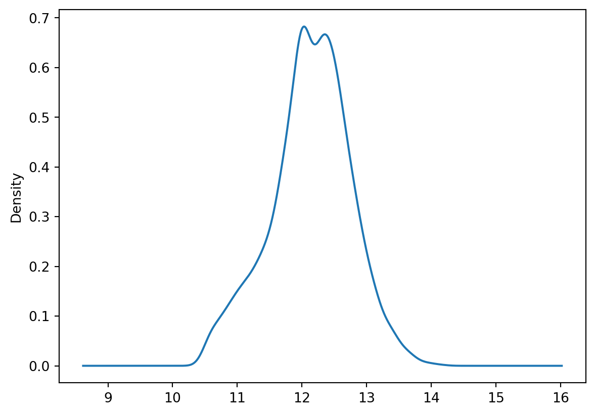
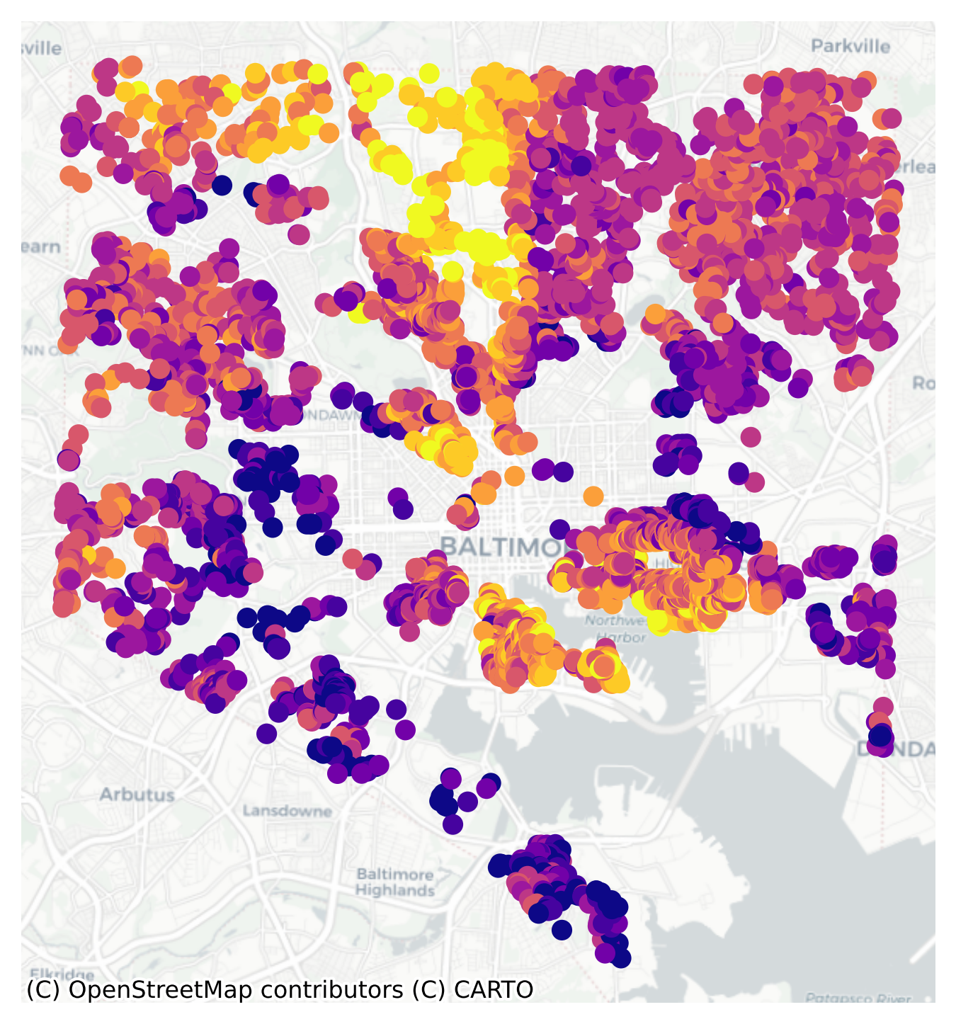
We generally start with ESDA (following the bottom-up strategy) to ensure we even care about spatial econometrics. We begin by mapping the dependent variable (housing price, here) and examining any global and local autocorrelation

Code
balt_sales[["considr1", "log_price", "geometry"]].explore(
    "log_price", scheme="fisher_jenks", k=10, cmap="plasma", tiles="CartoDB Positron"
)
Make this Notebook Trusted to load map: File -> Trust Notebook

There are definitely spatial patterns, but they’re also not uniform. There’s probably autocorrelation in the sales prices, but it seems to be particularly strong in some pockets. We should be sure to check both global and local statistics. As such, we need a spatial Graph object to define the relationship between housing sales, and we have seen in prior chapters the importance of considering travel network structure. Here we will fit two different graphs and examine global and local autocorrelation using both.

Code
w_dist = Graph.build_distance_band(balt_sales, threshold=1000)
w_dist = w_dist.transform("r")

w_net = Graph.build_travel_cost(balt_sales.to_crs(4326), balt_net, threshold=1000)
w_net = w_net.transform("r")

30.2.1 Global Stats

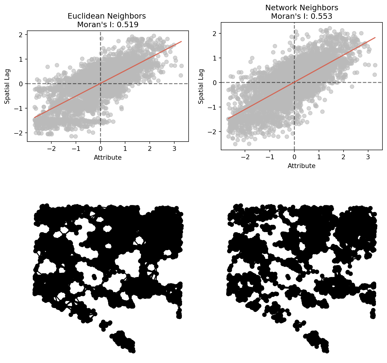
To check global autocorrelation we follow the same basic procedure, creating Moran objects for both types of Graph (to which we refer as \(W\), following the spatial econometric terminology).

Code
moran = esda.Moran(balt_sales["log_price"], w_dist)
moran_net = esda.Moran(balt_sales["log_price"], w_net)

f, ax = plt.subplots(2, 2, figsize=(10, 10))
ax = ax.flatten()
moran.plot_scatter(ax=ax[0])
moran_net.plot_scatter(ax=ax[1])

ax[0].set_title(f"Euclidean Neighbors \nMoran's I: {round(moran.I, 3)}")
ax[1].set_title(f"Network Neighbors\nMoran's I: {round(moran_net.I, 3)}")

w_dist.plot(balt_sales, ax=ax[2])
ax[2].axis("off")
w_net.plot(balt_sales, ax=ax[3])
ax[3].axis("off")

plt.tight_layout

For reference, we also plot the spatial structure of each graph below its Moran scatterplot. The comparison shows (as expected) that the network-based neighborhood results in more localized neighbor-sets and higher levels of autocorrelation (.55 versus .52).

30.2.2 Local Stats

And following, we will do the same with LISA plots of the local Moran statistics.

Code
lisa = esda.Moran_Local(
    balt_sales.log_price,
    w_net,
    n_jobs=-1,
)
ax = lisa.plot(balt_sales, alpha=0.7, figsize=(7, 7))
ax.axis("off")
ctx.add_basemap(ax=ax, source=ctx.providers.CartoDB.Positron, crs=balt_sales.crs)

The local Moran shows that our significant Moran statistic is driven by hotspots in “the Wedge” in the north-center of the city and the Inner Harbor, as well as coldspots in East and West Baltimore.

30.3 Models

Taking different modeling strategies, we can vary the way we operationalize \(p(h)\) to best identify the coefficients of interest, including the potential for spatial spillover (e.g. the price of one unit affecting the prices of those nearby). We specify the main parts of this model using Wilkinson formula, which is familiar if you have ever used R (Wilkinson & Rogers, 1973).

Here we will specify the log of sales price as a function of structural characteristics (size, age, dwelling type, construction type, and ‘structure grade’, as well as a squared age term to capture historic effects), demographic and socioeconomic attributes of the home’s census blockgroup, and its accessibility to jobs. A nice thing about Wilkinson formulas in formulaic is the ability to transform variables dynamically, thus here we set several variables as categorical (using the C() convention), and log-transform the square footage of the structure.

Code
formula = "log_price ~ 1 + STRUGRAD + C(RESITYP) + C(DESCCNST) + np.log(SQFTSTRC) + struc_age + age_square + p_nonhisp_white_persons + p_edu_college_greater + log_inc + p_housing_units_multiunit_structures + p_owner_occupied_units +  log_jobaccess"

30.3.1 Aspatial (OLS)

We will start by fitting the classic regression model which assumes observations are independent; in this case, that means the sales price of a home is dependent entirely on attributes of that home and is unaffected by homes nearby. We can start by fitting the model using the statsmodels package, which is the standard regression library in Python and provides a nice interface a builtin (classic) diagnostics.

\[y = \beta X + \epsilon\]

30.3.1.1 Using statsmodels

To proceed with statsmodels, we use the ols function from its ‘formula api’ (which is designed to accept Wilkinson formulas). The function returns an OLS class, upon which we call the fit method. Once the model is fit, the summary method returns a table of coefficients and model diagnostics.

Code
model_ols = smf.ols(formula, balt_sales).fit()
model_ols.summary()
OLS Regression Results
Dep. Variable: log_price R-squared: 0.709
Model: OLS Adj. R-squared: 0.708
Method: Least Squares F-statistic: 611.8
Date: Thu, 22 May 2025 Prob (F-statistic): 0.00
Time: 10:52:45 Log-Likelihood: -1767.8
No. Observations: 5543 AIC: 3582.
Df Residuals: 5520 BIC: 3734.
Df Model: 22
Covariance Type: nonrobust
coef std err t P>|t| [0.025 0.975]
Intercept 4.0446 0.237 17.083 0.000 3.580 4.509
C(RESITYP)[T.TH] -0.1506 0.014 -10.555 0.000 -0.179 -0.123
C(DESCCNST)[T.CNST 1/2 Brick Siding] -0.0465 0.079 -0.586 0.558 -0.202 0.109
C(DESCCNST)[T.CNST 1/2 Stone Frame] -0.4852 0.117 -4.135 0.000 -0.715 -0.255
C(DESCCNST)[T.CNST 1/2 Stone Siding] 0.4740 0.242 1.955 0.051 -0.001 0.949
C(DESCCNST)[T.CNST Block] -0.0026 0.072 -0.037 0.971 -0.144 0.139
C(DESCCNST)[T.CNST Brick] -0.0113 0.051 -0.220 0.826 -0.112 0.089
C(DESCCNST)[T.CNST Frame] -0.0148 0.052 -0.285 0.776 -0.117 0.087
C(DESCCNST)[T.CNST Shingle Asbestos] 0.1088 0.057 1.896 0.058 -0.004 0.221
C(DESCCNST)[T.CNST Shingle Wood] 0.0144 0.061 0.235 0.814 -0.105 0.134
C(DESCCNST)[T.CNST Siding] 0.0638 0.052 1.235 0.217 -0.037 0.165
C(DESCCNST)[T.CNST Stone] 0.1649 0.075 2.187 0.029 0.017 0.313
C(DESCCNST)[T.CNST Stucco] -0.0098 0.057 -0.172 0.864 -0.122 0.102
STRUGRAD 0.6925 0.025 27.730 0.000 0.644 0.741
np.log(SQFTSTRC) 0.5248 0.016 33.738 0.000 0.494 0.555
struc_age -0.0041 0.001 -7.942 0.000 -0.005 -0.003
age_square 1.613e-05 3.06e-06 5.272 0.000 1.01e-05 2.21e-05
p_nonhisp_white_persons -0.0003 0.000 -1.159 0.246 -0.001 0.000
p_edu_college_greater 0.0055 0.000 13.230 0.000 0.005 0.006
log_inc 0.2276 0.018 12.856 0.000 0.193 0.262
p_housing_units_multiunit_structures 0.0022 0.000 8.744 0.000 0.002 0.003
p_owner_occupied_units 0.0070 0.001 13.748 0.000 0.006 0.008
log_jobaccess 0.0366 0.005 6.671 0.000 0.026 0.047
Omnibus: 586.529 Durbin-Watson: 1.363
Prob(Omnibus): 0.000 Jarque-Bera (JB): 803.416
Skew: -0.851 Prob(JB): 3.47e-175
Kurtosis: 3.763 Cond. No. 5.99e+05


Notes:
[1] Standard Errors assume that the covariance matrix of the errors is correctly specified.
[2] The condition number is large, 5.99e+05. This might indicate that there are
strong multicollinearity or other numerical problems.


For a first shot, this is a decent model, with an \(R^2\) value greater than 0.7. Most of the variables are significant, except for the construction materials, in which only the siding has a significant effect. Otherwise, the coefficients are as expected. Housing prices increase with larger and newer homes (though historic homes also get a bump). Townhomes are less expensive than single family, and there are some small effects from the neighborhood’s demographic composition, the one exception being median income, which is relatively large.

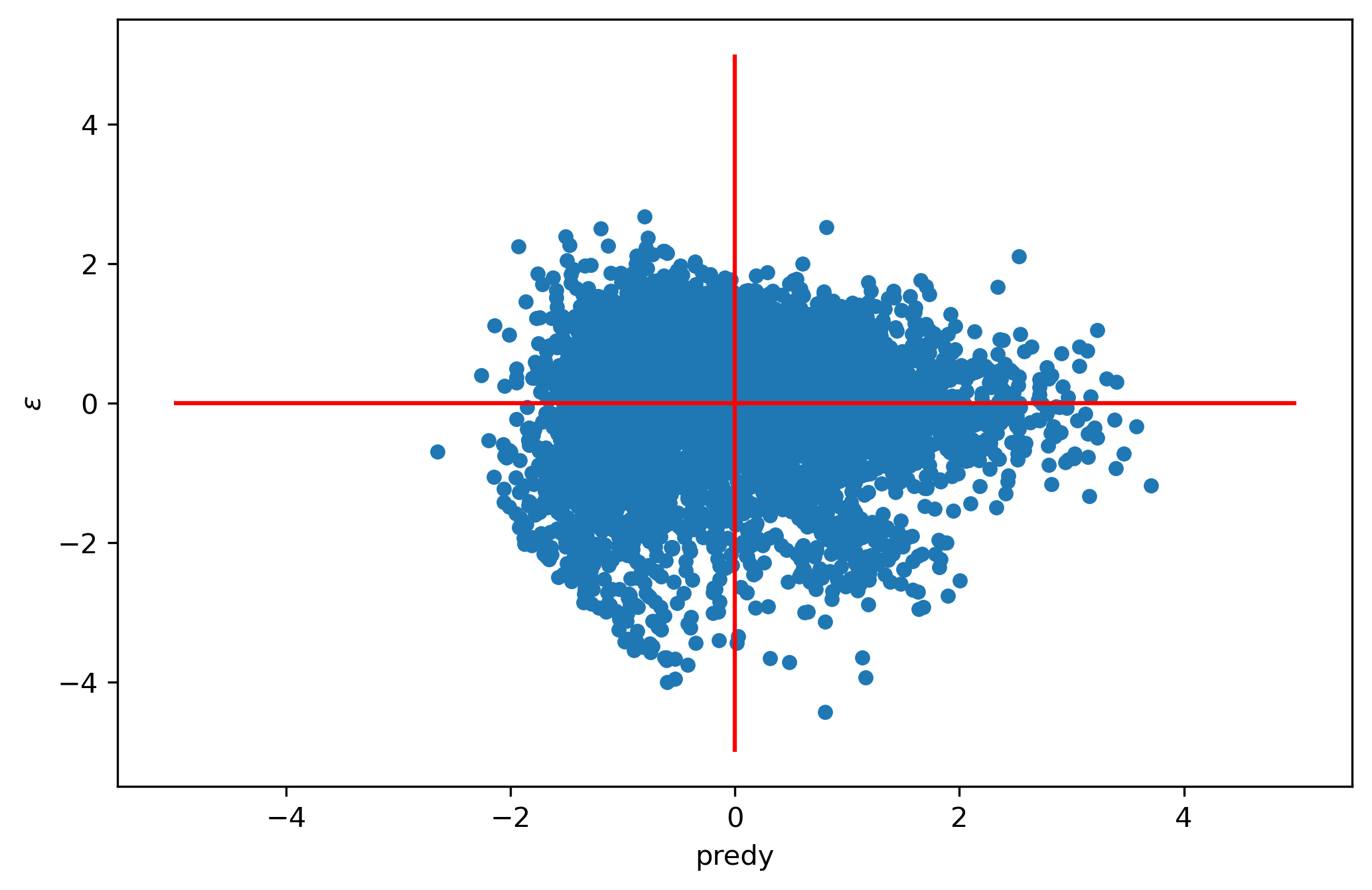
With linear regression models, among our primary concerns are that model residuals are independent and identically-distributed (I.I.D.). They do not necessarily need to be normal (though it’s ideal if they are), but they should be independent from one another (and ideally follow a known probability distribution). If the residuals are not identically-distributed, then robust errors can help insulate inferences, however the independence criterion is more difficult to handle. To check these criteria, it is common to plot the (standardized) predicted values against (standardized) residuals and visually assess randomness.

Code
ax = pd.DataFrame(
    {"predy": zscore(model_ols.fittedvalues), "$\epsilon$": zscore(model_ols.resid)}
).plot(x="predy", y="$\epsilon$", kind="scatter")
ax.hlines(0, -5, 5, "red")
ax.vlines(0, -5, 5, "red")
<>:2: SyntaxWarning: invalid escape sequence '\e'
<>:3: SyntaxWarning: invalid escape sequence '\e'
<>:2: SyntaxWarning: invalid escape sequence '\e'
<>:3: SyntaxWarning: invalid escape sequence '\e'
/var/folders/j8/5bgcw6hs7cqcbbz48d6bsftw0000gp/T/ipykernel_13809/2259918956.py:2: SyntaxWarning: invalid escape sequence '\e'
  {"predy": zscore(model_ols.fittedvalues), "$\epsilon$": zscore(model_ols.resid)}
/var/folders/j8/5bgcw6hs7cqcbbz48d6bsftw0000gp/T/ipykernel_13809/2259918956.py:3: SyntaxWarning: invalid escape sequence '\e'
  ).plot(x="predy", y="$\epsilon$", kind="scatter")

Code
ax = sns.kdeplot(y=zscore(model_ols.fittedvalues), x=zscore(model_ols.resid))
ax.hlines(0, -5, 5, 'red')
ax.vlines(0,-5, 5, 'red')

With this model the residuals are imperfect though not wholly unreasonable.

30.3.1.2 Using spreg

To generate spatial diagnostics for our model, we need to re-fit it using the spreg package from PySAL. However, since spreg does not understand Wilkinson formulas natively, we use the formulaic package, whose Formula class consumes a dataframe and the formula string, then returns the response vector and design matrix as spreg requires them. All other spatial specifications can be performed via options in the spreg estimation classes2.

Code
y, X = Formula(formula).get_model_matrix(pd.DataFrame(balt_sales))

Fitting this model using spreg we pass the y and X variables to the OLS class, but since we also want spatial diagnostics, we also include the Graph object (to the w argument), and include spat_diag=True which computes Lagrange Multiplier tests for spatial dependence in the residual3. Here we also compute the Moran test on the residuals, which requires an extra option given its additional computational overhead.

Code
model_ols_spreg = OLS(
    y=y,
    x=X,
    w=w_net,
    moran=True,
    spat_diag=True,
)

Once model is estimated using spreg, the coefficients and tests can be viewed

Code
print(model_ols_spreg.summary)
REGRESSION RESULTS
------------------

SUMMARY OF OUTPUT: ORDINARY LEAST SQUARES
-----------------------------------------
Data set            :     unknown
Weights matrix      :     unknown
Dependent Variable  :   log_price                Number of Observations:        5543
Mean dependent var  :     12.1398                Number of Variables   :          23
S.D. dependent var  :      0.6173                Degrees of Freedom    :        5520
R-squared           :      0.7092
Adjusted R-squared  :      0.7080
Sum squared residual:     614.167                F-statistic           :    611.8235
Sigma-square        :       0.111                Prob(F-statistic)     :           0
S.E. of regression  :       0.334                Log likelihood        :   -1767.807
Sigma-square ML     :       0.111                Akaike info criterion :    3581.614
S.E of regression ML:      0.3329                Schwarz criterion     :    3733.881

------------------------------------------------------------------------------------
            Variable     Coefficient       Std.Error     t-Statistic     Probability
------------------------------------------------------------------------------------
            CONSTANT         4.04459         0.23675        17.08350         0.00000
            STRUGRAD         0.69246         0.02497        27.72953         0.00000
    C(RESITYP)[T.TH]        -0.15059         0.01427       -10.55469         0.00000
C(DESCCNST)[T.CNST 1/2 Brick Siding]        -0.04646         0.07929        -0.58593         0.55795
C(DESCCNST)[T.CNST 1/2 Stone Frame]        -0.48521         0.11735        -4.13475         0.00004
C(DESCCNST)[T.CNST 1/2 Stone Siding]         0.47405         0.24243         1.95540         0.05059
C(DESCCNST)[T.CNST Block]        -0.00263         0.07200        -0.03656         0.97084
C(DESCCNST)[T.CNST Brick]        -0.01128         0.05129        -0.22000         0.82588
C(DESCCNST)[T.CNST Frame]        -0.01480         0.05196        -0.28482         0.77579
C(DESCCNST)[T.CNST Shingle Asbestos]         0.10879         0.05738         1.89607         0.05800
C(DESCCNST)[T.CNST Shingle Wood]         0.01438         0.06109         0.23547         0.81385
C(DESCCNST)[T.CNST Siding]         0.06378         0.05164         1.23502         0.21688
C(DESCCNST)[T.CNST Stone]         0.16493         0.07543         2.18656         0.02882
C(DESCCNST)[T.CNST Stucco]        -0.00981         0.05711        -0.17180         0.86360
    np.log(SQFTSTRC)         0.52480         0.01555        33.73850         0.00000
           struc_age        -0.00413         0.00052        -7.94159         0.00000
          age_square         0.00002         0.00000         5.27204         0.00000
p_nonhisp_white_persons        -0.00028         0.00024        -1.15927         0.24640
p_edu_college_greater         0.00547         0.00041        13.22992         0.00000
             log_inc         0.22761         0.01771        12.85557         0.00000
p_housing_units_multiunit_structures         0.00225         0.00026         8.74427         0.00000
p_owner_occupied_units         0.00701         0.00051        13.74775         0.00000
       log_jobaccess         0.03663         0.00549         6.67101         0.00000
------------------------------------------------------------------------------------
Warning: Variable(s) ['Intercept'] removed for being constant.

REGRESSION DIAGNOSTICS
MULTICOLLINEARITY CONDITION NUMBER         225.244

TEST ON NORMALITY OF ERRORS
TEST                             DF        VALUE           PROB
Jarque-Bera                       2        803.416           0.0000

DIAGNOSTICS FOR HETEROSKEDASTICITY
RANDOM COEFFICIENTS
TEST                             DF        VALUE           PROB
Breusch-Pagan test               22        656.878           0.0000
Koenker-Bassett test             22        475.417           0.0000

DIAGNOSTICS FOR SPATIAL DEPENDENCE
- SARERR -
TEST                           MI/DF       VALUE           PROB
Moran's I (error)              0.1570       27.192           0.0000
Lagrange Multiplier (lag)         1        259.451           0.0000
Robust LM (lag)                   1         49.536           0.0000
Lagrange Multiplier (error)       1        720.495           0.0000
Robust LM (error)                 1        510.580           0.0000
Lagrange Multiplier (SARMA)       2        770.032           0.0000

- Spatial Durbin -
TEST                              DF       VALUE           PROB
LM test for WX                   22        496.495           0.0000
Robust LM WX test                22        844.946           0.0000
Lagrange Multiplier (lag)         1        259.451           0.0000
Robust LM Lag - SDM               1        607.902           0.0000
Joint test for SDM               23       1104.397           0.0000
================================ END OF REPORT =====================================

The estimated model coefficients are the same between packages, but using spreg, we get a full suite of spatial diagnostics in the resulting summary, all of which are highly significant. These results show overwhelming evidence our model should account for some kind of spatial dependence, but since all the tests are significant, we need more exploration to understand which model is most appropriate. So we will step-up our spatial models one at a time, following Anselin (2007). Further, as with the statsmodels result, the Jarque-Bera test of normality on the residuals is highly significant, which could indicate we need to use a robust estimator.

30.3.2 Spatial Lag-of-X (SLX)

To fit an SLX model using the same spatial weights matrix for the dependent variable and every independent variable, you can simply use spreg’s OLS class and pass a Graph, and the argument slx_lags=1, which indicates that the model should include a \(WX\) variable for each of the explanatory variables in the model formula (design matrix). This fits the model:

\[y = \beta X + \theta WX + \epsilon\]

Code
model_slx = OLS(
    y=y,
    x=X,
    w=w_net,
    moran=True,
    spat_diag=True,
    slx_lags=1,
)
model_slx.output
var_names coefficients std_err zt_stat prob
0 CONSTANT 4.657921 0.275178 16.926912 0.0
1 STRUGRAD 0.656874 0.025777 25.482499 0.0
2 C(RESITYP)[T.TH] -0.1728 0.017017 -10.154294 0.0
3 C(DESCCNST)[T.CNST 1/2 Brick Siding] -0.038273 0.075952 -0.503912 0.614343
4 C(DESCCNST)[T.CNST 1/2 Stone Frame] -0.483672 0.112968 -4.281496 0.000019
5 C(DESCCNST)[T.CNST 1/2 Stone Siding] 0.346293 0.23223 1.491168 0.135975
6 C(DESCCNST)[T.CNST Block] -0.051904 0.069043 -0.751759 0.452228
7 C(DESCCNST)[T.CNST Brick] -0.02521 0.049199 -0.512396 0.608394
8 C(DESCCNST)[T.CNST Frame] -0.030854 0.049825 -0.61924 0.535784
9 C(DESCCNST)[T.CNST Shingle Asbestos] 0.046052 0.055211 0.834112 0.404254
10 C(DESCCNST)[T.CNST Shingle Wood] -0.024746 0.059089 -0.418798 0.67538
11 C(DESCCNST)[T.CNST Siding] 0.019695 0.0497 0.396283 0.691912
12 C(DESCCNST)[T.CNST Stone] 0.15744 0.073158 2.152063 0.031436
13 C(DESCCNST)[T.CNST Stucco] -0.03956 0.054792 -0.722 0.470325
14 np.log(SQFTSTRC) 0.542276 0.015926 34.049557 0.0
15 struc_age -0.004158 0.000541 -7.678068 0.0
16 age_square 0.000015 0.000003 4.575224 0.000005
17 p_nonhisp_white_persons 0.001509 0.000391 3.860529 0.000114
18 p_edu_college_greater 0.002251 0.000475 4.737025 0.000002
19 log_inc 0.14925 0.018049 8.269023 0.0
20 p_housing_units_multiunit_structures 0.001594 0.000291 5.480163 0.0
21 p_owner_occupied_units 0.003837 0.000573 6.695649 0.0
22 log_jobaccess 0.05092 0.01723 2.955358 0.003136
23 W_STRUGRAD 0.033285 0.051052 0.651985 0.514438
24 W_C(RESITYP)[T.TH] 0.071651 0.028967 2.47352 0.013409
25 W_C(DESCCNST)[T.CNST 1/2 Brick Siding] -1.101108 0.228329 -4.822467 0.000001
26 W_C(DESCCNST)[T.CNST 1/2 Stone Frame] -1.461694 0.289068 -5.056574 0.0
27 W_C(DESCCNST)[T.CNST 1/2 Stone Siding] 1.234218 1.029192 1.199211 0.230497
28 W_C(DESCCNST)[T.CNST Block] -0.9573 0.207069 -4.623095 0.000004
29 W_C(DESCCNST)[T.CNST Brick] -0.968864 0.155134 -6.245351 0.0
30 W_C(DESCCNST)[T.CNST Frame] -1.06164 0.156438 -6.786312 0.0
31 W_C(DESCCNST)[T.CNST Shingle Asbestos] -0.750257 0.171349 -4.37852 0.000012
32 W_C(DESCCNST)[T.CNST Shingle Wood] -1.154997 0.175167 -6.593674 0.0
33 W_C(DESCCNST)[T.CNST Siding] -0.785507 0.153236 -5.126132 0.0
34 W_C(DESCCNST)[T.CNST Stone] -1.060029 0.236464 -4.482833 0.000008
35 W_C(DESCCNST)[T.CNST Stucco] -0.878195 0.172098 -5.102881 0.0
36 W_np.log(SQFTSTRC) -0.137022 0.03084 -4.442984 0.000009
37 W_struc_age 0.002499 0.001116 2.240427 0.025103
38 W_age_square -0.00001 0.000007 -1.480908 0.138688
39 W_p_nonhisp_white_persons -0.004023 0.000492 -8.175412 0.0
40 W_p_edu_college_greater 0.005915 0.000695 8.509835 0.0
41 W_log_inc 0.131797 0.025514 5.165596 0.0
42 W_p_housing_units_multiunit_structures 0.001803 0.000522 3.455376 0.000554
43 W_p_owner_occupied_units 0.008587 0.000998 8.603926 0.0
44 W_log_jobaccess -0.019147 0.019066 -1.004258 0.315299

In addition to the summary attribute, which stores a large textual report, the output attribute of each spreg class stores the estimated coefficients and significance measures as a pandas DataFrame. In this output, we can see each of the \(X\) variables in the original specification now also has a \(WX\) version (prefixed by W_), many of which are significant. These results show clear and substantive evidence of spatial spillover (especially for neighborhood income W_loginc, which has a very large coefficient), where attributes of observations nearby influence the outcome at a different location.

Code
print(f"Robust LM Error p-value: {model_slx.rlm_error[1]}")
print(f"Robust LM Lag p-value: {model_slx.rlm_lag[1]}")
Robust LM Error p-value: 0.004444097228419605
Robust LM Lag p-value: 0.00017505329128955264

Despite significant \(WX\) results, the robust Lagrange Multiplier tests for both the SEM and SAR models are highly significant, showing significant autocorrelation remaining in the residual and suggesting we still need to explore more models.

30.3.3 Spatial Error (SEM)

To fit the spatial error model it is best to use the GMM_Error class, which fits the model:

\[y = \beta X + u\] \[ u = \lambda Wu+ \epsilon \]

Note

Classic estimation for spatial econometric models uses Maximum-Likelihood (ML), but modern applications typically prefer Generalized Method of Moments (GMM) for spatial error variants and Two-Stage Least Squares (TSLS) estimation for lag-based models, both of which are faster and applicable to larger datasets. Below, we will only use the spreg classes based on these estimators, however this is important to know, because TSLS estimation uses higher-order spatial lags of the X variables as instruments for estimating \(\rho WY\) by default. This will cause problems when estimating models that also include lagged \(X\)-variables (i.e. SLX-Error and Spatial Durbin). To avoid these errors, you can provide alternative instruments yourself, or you can pass w_lags >=2 which uses even higher-order neighbors as instruments.

Following the same conventions as above, we pass y, X, and W, then examine the output. Since the OLS model also showed some evidence of heteroskedasticity in the errors, we will also use a robust estimator by passing estimator="het".

Code
model_sem = GMM_Error(
    y=y,
    x=X,
    w=w_net,
    estimator="het",
)
model_sem.output.round(4)
var_names coefficients std_err zt_stat prob
0 CONSTANT 5.161013 0.264476 19.514136 0.0
1 STRUGRAD 0.688954 0.027537 25.018805 0.0
2 C(RESITYP)[T.TH] -0.176343 0.016622 -10.608905 0.0
3 C(DESCCNST)[T.CNST 1/2 Brick Siding] -0.000097 0.066132 -0.001459 0.998836
4 C(DESCCNST)[T.CNST 1/2 Stone Frame] -0.432683 0.143303 -3.019352 0.002533
5 C(DESCCNST)[T.CNST 1/2 Stone Siding] 0.36846 0.119828 3.074907 0.002106
6 C(DESCCNST)[T.CNST Block] 0.013489 0.066659 0.202355 0.839639
7 C(DESCCNST)[T.CNST Brick] 0.024513 0.045946 0.533529 0.593667
8 C(DESCCNST)[T.CNST Frame] 0.027819 0.046847 0.593822 0.552631
9 C(DESCCNST)[T.CNST Shingle Asbestos] 0.094486 0.049553 1.906755 0.056552
10 C(DESCCNST)[T.CNST Shingle Wood] 0.054446 0.052307 1.040898 0.297923
11 C(DESCCNST)[T.CNST Siding] 0.06578 0.046627 1.410793 0.158306
12 C(DESCCNST)[T.CNST Stone] 0.211491 0.05668 3.731341 0.00019
13 C(DESCCNST)[T.CNST Stucco] 0.011386 0.048705 0.233772 0.815162
14 np.log(SQFTSTRC) 0.533052 0.016739 31.844092 0.0
15 struc_age -0.00438 0.00043 -10.182988 0.0
16 age_square 0.000016 0.000003 6.472368 0.0
17 p_nonhisp_white_persons 0.001289 0.000347 3.710607 0.000207
18 p_edu_college_greater 0.004436 0.000493 9.002822 0.0
19 log_inc 0.141863 0.020014 7.088126 0.0
20 p_housing_units_multiunit_structures 0.001644 0.000276 5.959066 0.0
21 p_owner_occupied_units 0.004236 0.000616 6.874524 0.0
22 log_jobaccess 0.038429 0.009645 3.984353 0.000068
23 lambda 0.664089 0.017602 37.72874 0.0
Code
print(model_sem.summary)
REGRESSION RESULTS
------------------

SUMMARY OF OUTPUT: GM SPATIALLY WEIGHTED LEAST SQUARES (HET)
------------------------------------------------------------
Data set            :     unknown
Weights matrix      :     unknown
Dependent Variable  :   log_price                Number of Observations:        5543
Mean dependent var  :     12.1398                Number of Variables   :          23
S.D. dependent var  :      0.6173                Degrees of Freedom    :        5520
Pseudo R-squared    :      0.7025
N. of iterations    :           1                Step1c computed       :          No

------------------------------------------------------------------------------------
            Variable     Coefficient       Std.Error     z-Statistic     Probability
------------------------------------------------------------------------------------
            CONSTANT         5.16101         0.26448        19.51414         0.00000
            STRUGRAD         0.68895         0.02754        25.01881         0.00000
    C(RESITYP)[T.TH]        -0.17634         0.01662       -10.60891         0.00000
C(DESCCNST)[T.CNST 1/2 Brick Siding]        -0.00010         0.06613        -0.00146         0.99884
C(DESCCNST)[T.CNST 1/2 Stone Frame]        -0.43268         0.14330        -3.01935         0.00253
C(DESCCNST)[T.CNST 1/2 Stone Siding]         0.36846         0.11983         3.07491         0.00211
C(DESCCNST)[T.CNST Block]         0.01349         0.06666         0.20236         0.83964
C(DESCCNST)[T.CNST Brick]         0.02451         0.04595         0.53353         0.59367
C(DESCCNST)[T.CNST Frame]         0.02782         0.04685         0.59382         0.55263
C(DESCCNST)[T.CNST Shingle Asbestos]         0.09449         0.04955         1.90676         0.05655
C(DESCCNST)[T.CNST Shingle Wood]         0.05445         0.05231         1.04090         0.29792
C(DESCCNST)[T.CNST Siding]         0.06578         0.04663         1.41079         0.15831
C(DESCCNST)[T.CNST Stone]         0.21149         0.05668         3.73134         0.00019
C(DESCCNST)[T.CNST Stucco]         0.01139         0.04871         0.23377         0.81516
    np.log(SQFTSTRC)         0.53305         0.01674        31.84409         0.00000
           struc_age        -0.00438         0.00043       -10.18299         0.00000
          age_square         0.00002         0.00000         6.47237         0.00000
p_nonhisp_white_persons         0.00129         0.00035         3.71061         0.00021
p_edu_college_greater         0.00444         0.00049         9.00282         0.00000
             log_inc         0.14186         0.02001         7.08813         0.00000
p_housing_units_multiunit_structures         0.00164         0.00028         5.95907         0.00000
p_owner_occupied_units         0.00424         0.00062         6.87452         0.00000
       log_jobaccess         0.03843         0.00964         3.98435         0.00007
              lambda         0.66409         0.01760        37.72874         0.00000
------------------------------------------------------------------------------------
Warning: Variable(s) ['Intercept'] removed for being constant.
================================ END OF REPORT =====================================

In these results, we now have a lambda coefficient for our spatial error term, which is highly significant (and pretty large at 0.66). Most \(X\) variables related to the building structure are still significant, and now the neighborhood racial composition becomes significant. The rest of the significant coefficients have changed values a bit, for example the log_inc coefficient is reduced to 0.142 (down from 0.228 in the OLS model).

30.3.4 Spatial Lag (SAR)

To fit a spatial lag model the preferred approach is to use the GM_Lag class, which uses TSLS under the hood. If you have additional instruments to use, you can pass them to yend, but here we will adopt the default (which computes then uses \(WX\) as instruments). For robustness, we will also include White standard errors.

\[y = \rho W y + \beta X + \epsilon\]

Code
model_sar = GM_Lag(
    y=y,
    x=X,
    w=w_net,
    robust="white",
)
model_sar.output
var_names coefficients std_err zt_stat prob
0 CONSTANT 3.226568 0.365568 8.826187 0.0
1 STRUGRAD 0.66338 0.028293 23.446806 0.0
2 C(RESITYP)[T.TH] -0.145024 0.015332 -9.459168 0.0
3 C(DESCCNST)[T.CNST 1/2 Brick Siding] -0.035061 0.07168 -0.489129 0.62475
4 C(DESCCNST)[T.CNST 1/2 Stone Frame] -0.482857 0.147447 -3.274794 0.001057
5 C(DESCCNST)[T.CNST 1/2 Stone Siding] 0.439667 0.117774 3.733133 0.000189
6 C(DESCCNST)[T.CNST Block] -0.003551 0.067755 -0.052416 0.958197
7 C(DESCCNST)[T.CNST Brick] -0.004382 0.047774 -0.091733 0.92691
8 C(DESCCNST)[T.CNST Frame] -0.007347 0.048774 -0.150637 0.880262
9 C(DESCCNST)[T.CNST Shingle Asbestos] 0.107498 0.05137 2.092609 0.036384
10 C(DESCCNST)[T.CNST Shingle Wood] 0.007668 0.054731 0.140113 0.88857
11 C(DESCCNST)[T.CNST Siding] 0.062658 0.047973 1.306116 0.191513
12 C(DESCCNST)[T.CNST Stone] 0.154081 0.056785 2.713432 0.006659
13 C(DESCCNST)[T.CNST Stucco] -0.010339 0.051645 -0.200204 0.841321
14 np.log(SQFTSTRC) 0.509277 0.01695 30.04528 0.0
15 struc_age -0.00419 0.000402 -10.410229 0.0
16 age_square 0.000016 0.000002 6.762482 0.0
17 p_nonhisp_white_persons -0.000185 0.000254 -0.725947 0.467871
18 p_edu_college_greater 0.004669 0.000485 9.634843 0.0
19 log_inc 0.201339 0.021762 9.251868 0.0
20 p_housing_units_multiunit_structures 0.001889 0.000287 6.589082 0.0
21 p_owner_occupied_units 0.006502 0.00057 11.409809 0.0
22 log_jobaccess 0.031588 0.005725 5.517353 0.0
23 W_log_price 0.113879 0.037709 3.019926 0.002528

Compared to the SEM, this model has a slightly better model fit, and some of the coefficients have changed a bit. The spatial autoregressive parameter called W_dep_var in the report is relatively small but highly significant. Racial composition in the neighborhood is no longer significant, and the neighborhood income coefficient has increased again up to 0.20.

Code
print(model_sar.summary)
REGRESSION RESULTS
------------------

SUMMARY OF OUTPUT: SPATIAL TWO STAGE LEAST SQUARES
--------------------------------------------------
Data set            :     unknown
Weights matrix      :     unknown
Dependent Variable  :   log_price                Number of Observations:        5543
Mean dependent var  :     12.1398                Number of Variables   :          24
S.D. dependent var  :      0.6173                Degrees of Freedom    :        5519
Pseudo R-squared    :      0.7208
Spatial Pseudo R-squared:  0.7113

White Standard Errors
------------------------------------------------------------------------------------
            Variable     Coefficient       Std.Error     z-Statistic     Probability
------------------------------------------------------------------------------------
            CONSTANT         3.22657         0.36557         8.82619         0.00000
            STRUGRAD         0.66338         0.02829        23.44681         0.00000
    C(RESITYP)[T.TH]        -0.14502         0.01533        -9.45917         0.00000
C(DESCCNST)[T.CNST 1/2 Brick Siding]        -0.03506         0.07168        -0.48913         0.62475
C(DESCCNST)[T.CNST 1/2 Stone Frame]        -0.48286         0.14745        -3.27479         0.00106
C(DESCCNST)[T.CNST 1/2 Stone Siding]         0.43967         0.11777         3.73313         0.00019
C(DESCCNST)[T.CNST Block]        -0.00355         0.06776        -0.05242         0.95820
C(DESCCNST)[T.CNST Brick]        -0.00438         0.04777        -0.09173         0.92691
C(DESCCNST)[T.CNST Frame]        -0.00735         0.04877        -0.15064         0.88026
C(DESCCNST)[T.CNST Shingle Asbestos]         0.10750         0.05137         2.09261         0.03638
C(DESCCNST)[T.CNST Shingle Wood]         0.00767         0.05473         0.14011         0.88857
C(DESCCNST)[T.CNST Siding]         0.06266         0.04797         1.30612         0.19151
C(DESCCNST)[T.CNST Stone]         0.15408         0.05678         2.71343         0.00666
C(DESCCNST)[T.CNST Stucco]        -0.01034         0.05164        -0.20020         0.84132
    np.log(SQFTSTRC)         0.50928         0.01695        30.04528         0.00000
           struc_age        -0.00419         0.00040       -10.41023         0.00000
          age_square         0.00002         0.00000         6.76248         0.00000
p_nonhisp_white_persons        -0.00018         0.00025        -0.72595         0.46787
p_edu_college_greater         0.00467         0.00048         9.63484         0.00000
             log_inc         0.20134         0.02176         9.25187         0.00000
p_housing_units_multiunit_structures         0.00189         0.00029         6.58908         0.00000
p_owner_occupied_units         0.00650         0.00057        11.40981         0.00000
       log_jobaccess         0.03159         0.00573         5.51735         0.00000
         W_log_price         0.11388         0.03771         3.01993         0.00253
------------------------------------------------------------------------------------
Instrumented: W_log_price
Instruments: W_C(DESCCNST)[T.CNST 1/2 Brick Siding], W_C(DESCCNST)[T.CNST
             1/2 Stone Frame], W_C(DESCCNST)[T.CNST 1/2 Stone Siding],
             W_C(DESCCNST)[T.CNST Block], W_C(DESCCNST)[T.CNST Brick],
             W_C(DESCCNST)[T.CNST Frame], W_C(DESCCNST)[T.CNST Shingle
             Asbestos], W_C(DESCCNST)[T.CNST Shingle Wood],
             W_C(DESCCNST)[T.CNST Siding], W_C(DESCCNST)[T.CNST Stone],
             W_C(DESCCNST)[T.CNST Stucco], W_C(RESITYP)[T.TH], W_STRUGRAD,
             W_age_square, W_log_inc, W_log_jobaccess, W_np.log(SQFTSTRC),
             W_p_edu_college_greater,
             W_p_housing_units_multiunit_structures,
             W_p_nonhisp_white_persons, W_p_owner_occupied_units,
             W_struc_age
Warning: Variable(s) ['Intercept'] removed for being constant.

DIAGNOSTICS FOR SPATIAL DEPENDENCE
TEST                              DF         VALUE           PROB
Anselin-Kelejian Test             1        198.503           0.0000

SPATIAL LAG MODEL IMPACTS
Impacts computed using the 'simple' method.
            Variable         Direct        Indirect          Total
            STRUGRAD         0.6634          0.0853          0.7486
    C(RESITYP)[T.TH]        -0.1450         -0.0186         -0.1637
C(DESCCNST)[T.CNST 1/2 Brick Siding]        -0.0351         -0.0045         -0.0396
C(DESCCNST)[T.CNST 1/2 Stone Frame]        -0.4829         -0.0621         -0.5449
C(DESCCNST)[T.CNST 1/2 Stone Siding]         0.4397          0.0565          0.4962
C(DESCCNST)[T.CNST Block]        -0.0036         -0.0005         -0.0040
C(DESCCNST)[T.CNST Brick]        -0.0044         -0.0006         -0.0049
C(DESCCNST)[T.CNST Frame]        -0.0073         -0.0009         -0.0083
C(DESCCNST)[T.CNST Shingle Asbestos]         0.1075          0.0138          0.1213
C(DESCCNST)[T.CNST Shingle Wood]         0.0077          0.0010          0.0087
C(DESCCNST)[T.CNST Siding]         0.0627          0.0081          0.0707
C(DESCCNST)[T.CNST Stone]         0.1541          0.0198          0.1739
C(DESCCNST)[T.CNST Stucco]        -0.0103         -0.0013         -0.0117
    np.log(SQFTSTRC)         0.5093          0.0654          0.5747
           struc_age        -0.0042         -0.0005         -0.0047
          age_square         0.0000          0.0000          0.0000
p_nonhisp_white_persons        -0.0002         -0.0000         -0.0002
p_edu_college_greater         0.0047          0.0006          0.0053
             log_inc         0.2013          0.0259          0.2272
p_housing_units_multiunit_structures         0.0019          0.0002          0.0021
p_owner_occupied_units         0.0065          0.0008          0.0073
       log_jobaccess         0.0316          0.0041          0.0356
================================ END OF REPORT =====================================

The summary for models that include lagged dependent variables is also slightly different, as the end of the summary table now includes a set of impacts for each explanatory variable that show the direct, indirect, and total effects associated with each input. Thus we can see the total impact of neighborhood income is actually even higher at 0.23 after accounting for spillover effects. The Anselin-Kelejian test for spatial dependence is still significant in this model (@ Anselin & Kelejian, 1997), which suggests we may need to use an even more general model like the Spatial Durbin.

30.3.5 SLX-Error (SLXE / Durbin-Error)

To fit an SLXE model, we use the GMM_Error class once again, but this time pass slx_lags=1, which automatically handles the creation and inclusion of our \(WX\) variables.

Code
model_slxe = GMM_Error(
    y=y,
    x=X,
    w=w_net,
    slx_lags=1,
    estimator="het",
)
model_slxe.output
var_names coefficients std_err zt_stat prob
0 CONSTANT 5.237659 0.307527 17.031549 0.0
1 STRUGRAD 0.658802 0.027699 23.784444 0.0
2 C(RESITYP)[T.TH] -0.184412 0.016731 -11.02234 0.0
3 C(DESCCNST)[T.CNST 1/2 Brick Siding] -0.041202 0.073425 -0.561139 0.574702
4 C(DESCCNST)[T.CNST 1/2 Stone Frame] -0.483449 0.157716 -3.065313 0.002174
5 C(DESCCNST)[T.CNST 1/2 Stone Siding] 0.320895 0.161336 1.988984 0.046703
6 C(DESCCNST)[T.CNST Block] -0.038833 0.069633 -0.557675 0.577066
7 C(DESCCNST)[T.CNST Brick] -0.017774 0.049766 -0.357151 0.720979
8 C(DESCCNST)[T.CNST Frame] -0.021969 0.050732 -0.433041 0.664985
9 C(DESCCNST)[T.CNST Shingle Asbestos] 0.049259 0.053326 0.923726 0.355629
10 C(DESCCNST)[T.CNST Shingle Wood] -0.008636 0.055609 -0.155299 0.876586
11 C(DESCCNST)[T.CNST Siding] 0.027519 0.050107 0.549192 0.582873
12 C(DESCCNST)[T.CNST Stone] 0.162329 0.058653 2.767616 0.005647
13 C(DESCCNST)[T.CNST Stucco] -0.029523 0.053202 -0.554922 0.578948
14 np.log(SQFTSTRC) 0.530311 0.016905 31.370128 0.0
15 struc_age -0.004355 0.000422 -10.327532 0.0
16 age_square 0.000016 0.000002 6.312068 0.0
17 p_nonhisp_white_persons 0.00125 0.000378 3.309019 0.000936
18 p_edu_college_greater 0.002971 0.000491 6.055285 0.0
19 log_inc 0.125151 0.019429 6.441608 0.0
20 p_housing_units_multiunit_structures 0.001493 0.000271 5.501106 0.0
21 p_owner_occupied_units 0.0036 0.000599 6.007609 0.0
22 log_jobaccess 0.040912 0.01705 2.39953 0.016416
23 W_STRUGRAD 0.035277 0.059795 0.589967 0.555213
24 W_C(RESITYP)[T.TH] 0.038051 0.03713 1.024803 0.305456
25 W_C(DESCCNST)[T.CNST 1/2 Brick Siding] -0.766295 0.295839 -2.590245 0.009591
26 W_C(DESCCNST)[T.CNST 1/2 Stone Frame] -0.769452 0.543346 -1.416138 0.156735
27 W_C(DESCCNST)[T.CNST 1/2 Stone Siding] 0.485173 0.80681 0.601347 0.547609
28 W_C(DESCCNST)[T.CNST Block] -0.552524 0.307572 -1.796403 0.07243
29 W_C(DESCCNST)[T.CNST Brick] -0.575493 0.245681 -2.342437 0.019158
30 W_C(DESCCNST)[T.CNST Frame] -0.646834 0.24739 -2.614638 0.008932
31 W_C(DESCCNST)[T.CNST Shingle Asbestos] -0.534881 0.258877 -2.066157 0.038814
32 W_C(DESCCNST)[T.CNST Shingle Wood] -0.718847 0.27203 -2.642528 0.008229
33 W_C(DESCCNST)[T.CNST Siding] -0.464928 0.24442 -1.902171 0.057149
34 W_C(DESCCNST)[T.CNST Stone] -0.649945 0.323313 -2.010262 0.044403
35 W_C(DESCCNST)[T.CNST Stucco] -0.503749 0.257301 -1.957819 0.050251
36 W_np.log(SQFTSTRC) -0.127882 0.040552 -3.15355 0.001613
37 W_struc_age 0.00062 0.001261 0.491888 0.622798
38 W_age_square -0.000001 0.000007 -0.083142 0.933739
39 W_p_nonhisp_white_persons -0.003292 0.000606 -5.427691 0.0
40 W_p_edu_college_greater 0.005894 0.000899 6.553917 0.0
41 W_log_inc 0.091642 0.033655 2.722953 0.00647
42 W_p_housing_units_multiunit_structures 0.001157 0.000663 1.744539 0.081065
43 W_p_owner_occupied_units 0.007976 0.001504 5.305089 0.0
44 W_log_jobaccess -0.017689 0.021072 -0.839463 0.40121
45 lambda 0.504191 0.022161 22.751134 0.0
Code
print(model_slxe.summary)
REGRESSION RESULTS
------------------

SUMMARY OF OUTPUT: GM SPATIALLY WEIGHTED LEAST SQUARES (HET) WITH SLX (SLX-Error)
---------------------------------------------------------------------------------
Data set            :     unknown
Weights matrix      :     unknown
Dependent Variable  :   log_price                Number of Observations:        5543
Mean dependent var  :     12.1398                Number of Variables   :          45
S.D. dependent var  :      0.6173                Degrees of Freedom    :        5498
Pseudo R-squared    :      0.7334
N. of iterations    :           1                Step1c computed       :          No

------------------------------------------------------------------------------------
            Variable     Coefficient       Std.Error     z-Statistic     Probability
------------------------------------------------------------------------------------
            CONSTANT         5.23766         0.30753        17.03155         0.00000
            STRUGRAD         0.65880         0.02770        23.78444         0.00000
    C(RESITYP)[T.TH]        -0.18441         0.01673       -11.02234         0.00000
C(DESCCNST)[T.CNST 1/2 Brick Siding]        -0.04120         0.07342        -0.56114         0.57470
C(DESCCNST)[T.CNST 1/2 Stone Frame]        -0.48345         0.15772        -3.06531         0.00217
C(DESCCNST)[T.CNST 1/2 Stone Siding]         0.32089         0.16134         1.98898         0.04670
C(DESCCNST)[T.CNST Block]        -0.03883         0.06963        -0.55768         0.57707
C(DESCCNST)[T.CNST Brick]        -0.01777         0.04977        -0.35715         0.72098
C(DESCCNST)[T.CNST Frame]        -0.02197         0.05073        -0.43304         0.66499
C(DESCCNST)[T.CNST Shingle Asbestos]         0.04926         0.05333         0.92373         0.35563
C(DESCCNST)[T.CNST Shingle Wood]        -0.00864         0.05561        -0.15530         0.87659
C(DESCCNST)[T.CNST Siding]         0.02752         0.05011         0.54919         0.58287
C(DESCCNST)[T.CNST Stone]         0.16233         0.05865         2.76762         0.00565
C(DESCCNST)[T.CNST Stucco]        -0.02952         0.05320        -0.55492         0.57895
    np.log(SQFTSTRC)         0.53031         0.01690        31.37013         0.00000
           struc_age        -0.00435         0.00042       -10.32753         0.00000
          age_square         0.00002         0.00000         6.31207         0.00000
p_nonhisp_white_persons         0.00125         0.00038         3.30902         0.00094
p_edu_college_greater         0.00297         0.00049         6.05528         0.00000
             log_inc         0.12515         0.01943         6.44161         0.00000
p_housing_units_multiunit_structures         0.00149         0.00027         5.50111         0.00000
p_owner_occupied_units         0.00360         0.00060         6.00761         0.00000
       log_jobaccess         0.04091         0.01705         2.39953         0.01642
          W_STRUGRAD         0.03528         0.05979         0.58997         0.55521
  W_C(RESITYP)[T.TH]         0.03805         0.03713         1.02480         0.30546
W_C(DESCCNST)[T.CNST 1/2 Brick Siding]        -0.76629         0.29584        -2.59024         0.00959
W_C(DESCCNST)[T.CNST 1/2 Stone Frame]        -0.76945         0.54335        -1.41614         0.15674
W_C(DESCCNST)[T.CNST 1/2 Stone Siding]         0.48517         0.80681         0.60135         0.54761
W_C(DESCCNST)[T.CNST Block]        -0.55252         0.30757        -1.79640         0.07243
W_C(DESCCNST)[T.CNST Brick]        -0.57549         0.24568        -2.34244         0.01916
W_C(DESCCNST)[T.CNST Frame]        -0.64683         0.24739        -2.61464         0.00893
W_C(DESCCNST)[T.CNST Shingle Asbestos]        -0.53488         0.25888        -2.06616         0.03881
W_C(DESCCNST)[T.CNST Shingle Wood]        -0.71885         0.27203        -2.64253         0.00823
W_C(DESCCNST)[T.CNST Siding]        -0.46493         0.24442        -1.90217         0.05715
W_C(DESCCNST)[T.CNST Stone]        -0.64994         0.32331        -2.01026         0.04440
W_C(DESCCNST)[T.CNST Stucco]        -0.50375         0.25730        -1.95782         0.05025
  W_np.log(SQFTSTRC)        -0.12788         0.04055        -3.15355         0.00161
         W_struc_age         0.00062         0.00126         0.49189         0.62280
        W_age_square        -0.00000         0.00001        -0.08314         0.93374
W_p_nonhisp_white_persons        -0.00329         0.00061        -5.42769         0.00000
W_p_edu_college_greater         0.00589         0.00090         6.55392         0.00000
           W_log_inc         0.09164         0.03366         2.72295         0.00647
W_p_housing_units_multiunit_structures         0.00116         0.00066         1.74454         0.08107
W_p_owner_occupied_units         0.00798         0.00150         5.30509         0.00000
     W_log_jobaccess        -0.01769         0.02107        -0.83946         0.40121
              lambda         0.50419         0.02216        22.75113         0.00000
------------------------------------------------------------------------------------
Warning: Variable(s) ['Intercept'] removed for being constant.
================================ END OF REPORT =====================================

With this result, we have both a lambda coefficient (which remains significant and large, though a bit smaller) and a series of W_ coefficients as with the SLX specification.

30.3.6 Spatial Durbin (SDM)

Code
model_durbin = GM_Lag(
    y=y,
    x=X,
    w=w_net,
    slx_lags=1,
)
model_durbin.output
var_names coefficients std_err zt_stat prob
0 CONSTANT 4.386308 0.266731 16.444689 0.0
1 STRUGRAD 0.669529 0.024879 26.910909 0.0
2 C(RESITYP)[T.TH] -0.183922 0.016443 -11.185764 0.0
3 C(DESCCNST)[T.CNST 1/2 Brick Siding] -0.006329 0.073279 -0.086369 0.931173
4 C(DESCCNST)[T.CNST 1/2 Stone Frame] -0.475969 0.108882 -4.371436 0.000012
5 C(DESCCNST)[T.CNST 1/2 Stone Siding] 0.274234 0.223949 1.224537 0.22075
6 C(DESCCNST)[T.CNST Block] -0.016437 0.066647 -0.246634 0.805191
7 C(DESCCNST)[T.CNST Brick] 0.008464 0.047549 0.178008 0.858717
8 C(DESCCNST)[T.CNST Frame] 0.009433 0.048205 0.195674 0.844866
9 C(DESCCNST)[T.CNST Shingle Asbestos] 0.057944 0.053227 1.088617 0.276323
10 C(DESCCNST)[T.CNST Shingle Wood] 0.014516 0.057098 0.254224 0.799322
11 C(DESCCNST)[T.CNST Siding] 0.041765 0.047956 0.870901 0.383808
12 C(DESCCNST)[T.CNST Stone] 0.187489 0.070579 2.656422 0.007897
13 C(DESCCNST)[T.CNST Stucco] -0.015917 0.052867 -0.301081 0.763353
14 np.log(SQFTSTRC) 0.551688 0.015381 35.868103 0.0
15 struc_age -0.004109 0.000522 -7.871901 0.0
16 age_square 0.000014 0.000003 4.589105 0.000004
17 p_nonhisp_white_persons 0.001861 0.000378 4.917092 0.000001
18 p_edu_college_greater 0.002241 0.000458 4.891937 0.000001
19 log_inc 0.144917 0.017402 8.327709 0.0
20 p_housing_units_multiunit_structures 0.001544 0.00028 5.503491 0.0
21 p_owner_occupied_units 0.003147 0.000557 5.650023 0.0
22 log_jobaccess 0.072764 0.016762 4.34103 0.000014
23 W_STRUGRAD -0.442253 0.069927 -6.324515 0.0
24 W_C(RESITYP)[T.TH] 0.115106 0.028285 4.069488 0.000047
25 W_C(DESCCNST)[T.CNST 1/2 Brick Siding] -0.901737 0.221047 -4.07939 0.000045
26 W_C(DESCCNST)[T.CNST 1/2 Stone Frame] -0.481457 0.296833 -1.62198 0.104808
27 W_C(DESCCNST)[T.CNST 1/2 Stone Siding] -1.380083 1.028858 -1.341374 0.179799
28 W_C(DESCCNST)[T.CNST Block] -0.778951 0.200441 -3.88618 0.000102
29 W_C(DESCCNST)[T.CNST Brick] -0.787185 0.150718 -5.222899 0.0
30 W_C(DESCCNST)[T.CNST Frame] -0.844437 0.152474 -5.538244 0.0
31 W_C(DESCCNST)[T.CNST Shingle Asbestos] -0.86509 0.165582 -5.224544 0.0
32 W_C(DESCCNST)[T.CNST Shingle Wood] -0.850145 0.171805 -4.948317 0.000001
33 W_C(DESCCNST)[T.CNST Siding] -0.766143 0.147703 -5.187067 0.0
34 W_C(DESCCNST)[T.CNST Stone] -0.85979 0.228862 -3.7568 0.000172
35 W_C(DESCCNST)[T.CNST Stucco] -0.678597 0.167174 -4.059229 0.000049
36 W_np.log(SQFTSTRC) -0.572687 0.054365 -10.534069 0.0
37 W_struc_age 0.002807 0.001076 2.609441 0.009069
38 W_age_square -0.000008 0.000006 -1.189759 0.234141
39 W_p_nonhisp_white_persons -0.002741 0.000493 -5.561842 0.0
40 W_p_edu_college_greater 0.003196 0.000728 4.391756 0.000011
41 W_log_inc -0.237469 0.045753 -5.190263 0.0
42 W_p_housing_units_multiunit_structures -0.001234 0.000594 -2.075322 0.037957
43 W_p_owner_occupied_units -0.00079 0.001373 -0.575707 0.564813
44 W_log_jobaccess -0.085574 0.019643 -4.356469 0.000013
45 W_log_price 0.759424 0.079348 9.57082 0.0
Code
print(model_durbin.summary)
REGRESSION RESULTS
------------------

SUMMARY OF OUTPUT: SPATIAL TWO STAGE LEAST SQUARES WITH SLX (SPATIAL DURBIN MODEL)
----------------------------------------------------------------------------------
Data set            :     unknown
Weights matrix      :     unknown
Dependent Variable  :   log_price                Number of Observations:        5543
Mean dependent var  :     12.1398                Number of Variables   :          46
S.D. dependent var  :      0.6173                Degrees of Freedom    :        5497
Pseudo R-squared    :      0.7521
Spatial Pseudo R-squared:  0.7122

------------------------------------------------------------------------------------
            Variable     Coefficient       Std.Error     z-Statistic     Probability
------------------------------------------------------------------------------------
            CONSTANT         4.38631         0.26673        16.44469         0.00000
            STRUGRAD         0.66953         0.02488        26.91091         0.00000
    C(RESITYP)[T.TH]        -0.18392         0.01644       -11.18576         0.00000
C(DESCCNST)[T.CNST 1/2 Brick Siding]        -0.00633         0.07328        -0.08637         0.93117
C(DESCCNST)[T.CNST 1/2 Stone Frame]        -0.47597         0.10888        -4.37144         0.00001
C(DESCCNST)[T.CNST 1/2 Stone Siding]         0.27423         0.22395         1.22454         0.22075
C(DESCCNST)[T.CNST Block]        -0.01644         0.06665        -0.24663         0.80519
C(DESCCNST)[T.CNST Brick]         0.00846         0.04755         0.17801         0.85872
C(DESCCNST)[T.CNST Frame]         0.00943         0.04821         0.19567         0.84487
C(DESCCNST)[T.CNST Shingle Asbestos]         0.05794         0.05323         1.08862         0.27632
C(DESCCNST)[T.CNST Shingle Wood]         0.01452         0.05710         0.25422         0.79932
C(DESCCNST)[T.CNST Siding]         0.04177         0.04796         0.87090         0.38381
C(DESCCNST)[T.CNST Stone]         0.18749         0.07058         2.65642         0.00790
C(DESCCNST)[T.CNST Stucco]        -0.01592         0.05287        -0.30108         0.76335
    np.log(SQFTSTRC)         0.55169         0.01538        35.86810         0.00000
           struc_age        -0.00411         0.00052        -7.87190         0.00000
          age_square         0.00001         0.00000         4.58910         0.00000
p_nonhisp_white_persons         0.00186         0.00038         4.91709         0.00000
p_edu_college_greater         0.00224         0.00046         4.89194         0.00000
             log_inc         0.14492         0.01740         8.32771         0.00000
p_housing_units_multiunit_structures         0.00154         0.00028         5.50349         0.00000
p_owner_occupied_units         0.00315         0.00056         5.65002         0.00000
       log_jobaccess         0.07276         0.01676         4.34103         0.00001
          W_STRUGRAD        -0.44225         0.06993        -6.32451         0.00000
  W_C(RESITYP)[T.TH]         0.11511         0.02829         4.06949         0.00005
W_C(DESCCNST)[T.CNST 1/2 Brick Siding]        -0.90174         0.22105        -4.07939         0.00005
W_C(DESCCNST)[T.CNST 1/2 Stone Frame]        -0.48146         0.29683        -1.62198         0.10481
W_C(DESCCNST)[T.CNST 1/2 Stone Siding]        -1.38008         1.02886        -1.34137         0.17980
W_C(DESCCNST)[T.CNST Block]        -0.77895         0.20044        -3.88618         0.00010
W_C(DESCCNST)[T.CNST Brick]        -0.78719         0.15072        -5.22290         0.00000
W_C(DESCCNST)[T.CNST Frame]        -0.84444         0.15247        -5.53824         0.00000
W_C(DESCCNST)[T.CNST Shingle Asbestos]        -0.86509         0.16558        -5.22454         0.00000
W_C(DESCCNST)[T.CNST Shingle Wood]        -0.85015         0.17180        -4.94832         0.00000
W_C(DESCCNST)[T.CNST Siding]        -0.76614         0.14770        -5.18707         0.00000
W_C(DESCCNST)[T.CNST Stone]        -0.85979         0.22886        -3.75680         0.00017
W_C(DESCCNST)[T.CNST Stucco]        -0.67860         0.16717        -4.05923         0.00005
  W_np.log(SQFTSTRC)        -0.57269         0.05437       -10.53407         0.00000
         W_struc_age         0.00281         0.00108         2.60944         0.00907
        W_age_square        -0.00001         0.00001        -1.18976         0.23414
W_p_nonhisp_white_persons        -0.00274         0.00049        -5.56184         0.00000
W_p_edu_college_greater         0.00320         0.00073         4.39176         0.00001
           W_log_inc        -0.23747         0.04575        -5.19026         0.00000
W_p_housing_units_multiunit_structures        -0.00123         0.00059        -2.07532         0.03796
W_p_owner_occupied_units        -0.00079         0.00137        -0.57571         0.56481
     W_log_jobaccess        -0.08557         0.01964        -4.35647         0.00001
         W_log_price         0.75942         0.07935         9.57082         0.00000
------------------------------------------------------------------------------------
Instrumented: W_log_price
Instruments: W2_C(DESCCNST)[T.CNST 1/2 Brick Siding], W2_C(DESCCNST)[T.CNST
             1/2 Stone Frame], W2_C(DESCCNST)[T.CNST 1/2 Stone Siding],
             W2_C(DESCCNST)[T.CNST Block], W2_C(DESCCNST)[T.CNST Brick],
             W2_C(DESCCNST)[T.CNST Frame], W2_C(DESCCNST)[T.CNST Shingle
             Asbestos], W2_C(DESCCNST)[T.CNST Shingle Wood],
             W2_C(DESCCNST)[T.CNST Siding], W2_C(DESCCNST)[T.CNST Stone],
             W2_C(DESCCNST)[T.CNST Stucco], W2_C(RESITYP)[T.TH],
             W2_STRUGRAD, W2_age_square, W2_log_inc, W2_log_jobaccess,
             W2_np.log(SQFTSTRC), W2_p_edu_college_greater,
             W2_p_housing_units_multiunit_structures,
             W2_p_nonhisp_white_persons, W2_p_owner_occupied_units,
             W2_struc_age
Warning: Variable(s) ['Intercept'] removed for being constant.

DIAGNOSTICS FOR SPATIAL DEPENDENCE
TEST                              DF         VALUE           PROB
Anselin-Kelejian Test             1         36.382           0.0000
Common Factor Hypothesis Test    22        303.684           0.0000

SPATIAL DURBIN MODEL IMPACTS
Impacts computed using the 'simple' method.
            Variable         Direct        Indirect          Total
            STRUGRAD         0.6695          0.2752          0.9447
    C(RESITYP)[T.TH]        -0.1839         -0.1021         -0.2860
C(DESCCNST)[T.CNST 1/2 Brick Siding]        -0.0063         -3.7682         -3.7745
C(DESCCNST)[T.CNST 1/2 Stone Frame]        -0.4760         -3.5038         -3.9797
C(DESCCNST)[T.CNST 1/2 Stone Siding]         0.2742         -4.8709         -4.5967
C(DESCCNST)[T.CNST Block]        -0.0164         -3.2897         -3.3062
C(DESCCNST)[T.CNST Brick]         0.0085         -3.2454         -3.2369
C(DESCCNST)[T.CNST Frame]         0.0094         -3.4803         -3.4709
C(DESCCNST)[T.CNST Shingle Asbestos]         0.0579         -3.4130         -3.3551
C(DESCCNST)[T.CNST Shingle Wood]         0.0145         -3.4880         -3.4735
C(DESCCNST)[T.CNST Siding]         0.0418         -3.0528         -3.0110
C(DESCCNST)[T.CNST Stone]         0.1875         -2.9820         -2.7945
C(DESCCNST)[T.CNST Stucco]        -0.0159         -2.8710         -2.8869
    np.log(SQFTSTRC)         0.5517         -0.6390         -0.0873
           struc_age        -0.0041         -0.0013         -0.0054
          age_square         0.0000          0.0000          0.0000
p_nonhisp_white_persons         0.0019         -0.0055         -0.0037
p_edu_college_greater         0.0022          0.0204          0.0226
             log_inc         0.1449         -0.5296         -0.3847
p_housing_units_multiunit_structures         0.0015         -0.0003          0.0013
p_owner_occupied_units         0.0031          0.0066          0.0098
       log_jobaccess         0.0728         -0.1260         -0.0532
================================ END OF REPORT =====================================

Notice in the report for the Durbin model the instrumented variable (W_dep_var) is estimated using instruments prefixed with W2_ indicating second-order spatial lags of the explanatory variables. That is, the GM_Lag class noticed we included slx_lags=1 and automatically incremented the order of \(WX\) to use as instruments. Obviously, you can modify this behavior or pass your own instruments if desired.

30.3.7 Comparison

Sometimes it can be useful to compare the estimated coefficients from each model side-by-side, but until now we’ve had them each in separate summaries. For simplicity, we can concatenate the output tables from each of the models, and we can make sure everything stays aligned by setting the variable as an index.

Code
pd.concat(
    [
        model_durbin.output.set_index("var_names")["coefficients"].rename("durbin"),
        model_slxe.output.set_index("var_names")["coefficients"].rename("slxe"),
        model_sar.output.set_index("var_names")["coefficients"].rename("lag"),
        model_sem.output.set_index("var_names")["coefficients"].rename("sem"),
        model_slx.output.set_index("var_names")["coefficients"].rename("slx"),
        model_ols_spreg.output.set_index("var_names")["coefficients"].rename("ols"),
    ],
    axis=1,
)
durbin slxe lag sem slx ols
var_names
CONSTANT 4.386308 5.237659 3.226568 5.161013 4.657921 4.04459
STRUGRAD 0.669529 0.658802 0.66338 0.688954 0.656874 0.692456
C(RESITYP)[T.TH] -0.183922 -0.184412 -0.145024 -0.176343 -0.1728 -0.150589
C(DESCCNST)[T.CNST 1/2 Brick Siding] -0.006329 -0.041202 -0.035061 -0.000097 -0.038273 -0.046456
C(DESCCNST)[T.CNST 1/2 Stone Frame] -0.475969 -0.483449 -0.482857 -0.432683 -0.483672 -0.485211
C(DESCCNST)[T.CNST 1/2 Stone Siding] 0.274234 0.320895 0.439667 0.36846 0.346293 0.474046
C(DESCCNST)[T.CNST Block] -0.016437 -0.038833 -0.003551 0.013489 -0.051904 -0.002632
C(DESCCNST)[T.CNST Brick] 0.008464 -0.017774 -0.004382 0.024513 -0.02521 -0.011285
C(DESCCNST)[T.CNST Frame] 0.009433 -0.021969 -0.007347 0.027819 -0.030854 -0.014799
C(DESCCNST)[T.CNST Shingle Asbestos] 0.057944 0.049259 0.107498 0.094486 0.046052 0.108793
C(DESCCNST)[T.CNST Shingle Wood] 0.014516 -0.008636 0.007668 0.054446 -0.024746 0.014384
C(DESCCNST)[T.CNST Siding] 0.041765 0.027519 0.062658 0.06578 0.019695 0.06378
C(DESCCNST)[T.CNST Stone] 0.187489 0.162329 0.154081 0.211491 0.15744 0.164929
C(DESCCNST)[T.CNST Stucco] -0.015917 -0.029523 -0.010339 0.011386 -0.03956 -0.009811
np.log(SQFTSTRC) 0.551688 0.530311 0.509277 0.533052 0.542276 0.524796
struc_age -0.004109 -0.004355 -0.00419 -0.00438 -0.004158 -0.004131
age_square 0.000014 0.000016 0.000016 0.000016 0.000015 0.000016
p_nonhisp_white_persons 0.001861 0.00125 -0.000185 0.001289 0.001509 -0.000279
p_edu_college_greater 0.002241 0.002971 0.004669 0.004436 0.002251 0.005473
log_inc 0.144917 0.125151 0.201339 0.141863 0.14925 0.227612
p_housing_units_multiunit_structures 0.001544 0.001493 0.001889 0.001644 0.001594 0.002245
p_owner_occupied_units 0.003147 0.0036 0.006502 0.004236 0.003837 0.007009
log_jobaccess 0.072764 0.040912 0.031588 0.038429 0.05092 0.036633
W_STRUGRAD -0.442253 0.035277 NaN NaN 0.033285 NaN
W_C(RESITYP)[T.TH] 0.115106 0.038051 NaN NaN 0.071651 NaN
W_C(DESCCNST)[T.CNST 1/2 Brick Siding] -0.901737 -0.766295 NaN NaN -1.101108 NaN
W_C(DESCCNST)[T.CNST 1/2 Stone Frame] -0.481457 -0.769452 NaN NaN -1.461694 NaN
W_C(DESCCNST)[T.CNST 1/2 Stone Siding] -1.380083 0.485173 NaN NaN 1.234218 NaN
W_C(DESCCNST)[T.CNST Block] -0.778951 -0.552524 NaN NaN -0.9573 NaN
W_C(DESCCNST)[T.CNST Brick] -0.787185 -0.575493 NaN NaN -0.968864 NaN
W_C(DESCCNST)[T.CNST Frame] -0.844437 -0.646834 NaN NaN -1.06164 NaN
W_C(DESCCNST)[T.CNST Shingle Asbestos] -0.86509 -0.534881 NaN NaN -0.750257 NaN
W_C(DESCCNST)[T.CNST Shingle Wood] -0.850145 -0.718847 NaN NaN -1.154997 NaN
W_C(DESCCNST)[T.CNST Siding] -0.766143 -0.464928 NaN NaN -0.785507 NaN
W_C(DESCCNST)[T.CNST Stone] -0.85979 -0.649945 NaN NaN -1.060029 NaN
W_C(DESCCNST)[T.CNST Stucco] -0.678597 -0.503749 NaN NaN -0.878195 NaN
W_np.log(SQFTSTRC) -0.572687 -0.127882 NaN NaN -0.137022 NaN
W_struc_age 0.002807 0.00062 NaN NaN 0.002499 NaN
W_age_square -0.000008 -0.000001 NaN NaN -0.00001 NaN
W_p_nonhisp_white_persons -0.002741 -0.003292 NaN NaN -0.004023 NaN
W_p_edu_college_greater 0.003196 0.005894 NaN NaN 0.005915 NaN
W_log_inc -0.237469 0.091642 NaN NaN 0.131797 NaN
W_p_housing_units_multiunit_structures -0.001234 0.001157 NaN NaN 0.001803 NaN
W_p_owner_occupied_units -0.00079 0.007976 NaN NaN 0.008587 NaN
W_log_jobaccess -0.085574 -0.017689 NaN NaN -0.019147 NaN
W_log_price 0.759424 NaN 0.113879 NaN NaN NaN
lambda NaN 0.504191 NaN 0.664089 NaN NaN

These models have different sets of terms (e.g. only SEM variants have lambda, only SLX variants have W_ variables, and only Lag variants have W_dep_var), so models missing the necessary coefficients will have NAs. Also remember that we’re joining together only the output from the lag models, not the impacts, so we are ignoring the indirect effects from these models.

Comparing the estimated coefficients shows that median income was doing a lot of heavy lifting in the OLS model. That is, when we ignore spatial effects, the median income variable absorbs a lot of the spatial variance, inflating its coefficient and biasing our interpretation of how much residents value higher-income neighbors. In the spatial models, the estimated coefficient for income is less than half as large. That’s basically true of all the other neighborhood characteristics as well.

Remember that our data are measured at two different spatial levels. Our housing sales are measured at the unit level, but the ‘neighborhood’ variables are measured at the census blockgroup level. Because we have several sales nested inside each census unit, we are building spatial autocorrelation into the model by design. That is, because we don’t know the income, education, race, etc of the home’s previous owner, the “neighborhood” variables coming from the Census are defined in geographic zones which are essentially \(WX\) instead of just \(X\), where \(W\) is defined by discrete membership inside a census unit.

30.5 Extensions

The spreg package also includes a wide variety of additional models we do not explore here, including spatial Seemingly Unrelated Regression (SUR), spatial Panel models (Elhorst, 2003, 2014), and diagnostics for Probit and non-linear models.

30.5.1 Regimes

In all of the examples above, we assume the relationship between \(X\) and \(y\) is constant over space. In some applications, however, there may be reason to believe that coefficients vary over the study region, i.e. there are different “treatment regimes” (Imai & van Dyk, 2004). Rather than estimate a separate regression for every data point a-la GWR, one way to handle spatially-varying relationships in a spatial econometric framework is through the use of spatial regimes which separate the study region into discrete portions (defined by a different \(W\) matrix), then fit separate models for each portion (Durlauf & Johnson, 1995). This is a bit like the geographic version of piecewise regression, where geographic zones are used to define the breakpoints rather than ranges of the outcome variable. Each of the models above optionally takes a regime argument that defines the grouping for each observation. Alternatively, spreg also offers a function for determining optimal regimes endogenously by combining SKATER constrained clustering with spatial regression, following Anselin & Amaral (2023).

30.5.2 Quasi Experiments and Causal Designs

A prominent critique of applied spatial econometric modeling is given by Gibbons & Overman (2012), who argue that the suite of models above

does not provide a toolbox that gives satisfactory solutions to these problems for applied researchers interested in causality and the economic processes at work. It is in this sense that we call into question the approach of the burgeoning body of applied economic research that proceeds with mechanical application of spatial econometric techniques to causal questions of “spillovers” and other forms of spatial interaction, or that estimates spatial lag models as a quick fix for endogeneity issues, or that blindly applies spatial econometric models by default without serious consideration of whether this is necessary given the research question in hand.

To overcome these issues, they argue that applied work should adopt what they term ‘experimentalist’ design4, where some form of exogenous variation is induced to provide insight into a causal mechanism at play. Spatial econometric models that incorporate quasi experimental designs are an active area of research, with early pioneering work by Dubé et al. (2014), Delgado & Florax (2015), Bardaka et al. (2018), and Diao et al. (2017), who blend different spatial specification above with a difference-in-differences framework. While this work represents an important step forward from traditional designs that ignore spatial dependence altogether, the complexity involved with DID designs that include spatial terms is still under-appreciated, and many important issues in urban policy analysis do not have a satisfactory specification using such an approach (Knaap, 2024).

Alternatively, structural models5 should proceed by considering the SLX model as the point of depatrture, or use strong theory to guide the choice of a particular specification as described above (Halleck Vega & Elhorst, 2015). Although there remains debate in urban economics, I believe there is a good justification for assuming a potential autoregressive process in the specific context of hedonic housing price models.


  1. Despite the preferences of LeSage & Pace (2009), Anselin et al. (2024) use the reduced form of the unrestricted SDM to show that “there is no solid theoretical basis for preferring one specification over the other, only an empirical one.”↩︎

  2. Using different arguments in the spreg classes allows one to fit all of the models described in previous sections, and the Wilkinson formula need not be changed for these specifications. It is also possible to fit increasingly complex models, e.g. where different explanatory variables are defined by different spatial scopes (\(W_1X_1, W_2 X_2\), etc.) (Galster, 2019), but these kinds of specifications need to be created manually e.g. by creating \(WX\) variables on the dataframe using the Graph.lag(x) convention. In this case, a user would want to specify these terms directly in Wilkinson formulas, and avoid using the slx_vars argument in spreg which applies the same Graph specification to each \(X\) variable.↩︎

  3. For a deep dive on computing specification tests, see Anselin et al. (1996) and the spreg documentation at https://pysal.org/spreg/notebooks/9_specification_tests.html↩︎

  4. Today this is more commonly called the “potential outcomes” framework (Rubin, 2005).↩︎

  5. Today I think econometricians prefer to call this “‘design-based’ inference” rather than “structural estimation” (Abadie et al., 2020; Borusyak et al., 2024; Manski & McFadden, 1981; Witte et al., 1979).↩︎