Code
import contextily as ctx
import geopandas as gpd
import matplotlib.pyplot as plt
import pandas as pd
from pointpats import Knox, KnoxLocal, plot_densityimport contextily as ctx
import geopandas as gpd
import matplotlib.pyplot as plt
import pandas as pd
from pointpats import Knox, KnoxLocal, plot_densityA classic tradition in spatial analysis examines the clustering of events in time and space. A set of “events” in this case is a dataset with both a geographic location (i.e. a point with X and Y coordinates) and a temporal location (i.e. a timestamp or some record of when something occurred). Events that cluster together in time and space can often be substantively important across a wide variety of social, behavioral, and natural sciences. For example in epidemiology, a cluster of events may help identify a disease outbreak, but understanding clustering in space-time event data is widely applicable in many fields. Further, the data are often already present in the most useful format. Example research questions and geocoded/timestamped data might include:
public health & epidemiology, e.g. to describe outbreaks or help identify inflection points in an epidemic
transportation, e.g. to identify dangerous intersections or high-demand transit locations
housing e.g. to identify transitioning land markets or residential displacement
marketing e.g. to understand which campaigns do better in which locations
criminology e.g. to understand inequality in police enforcement or victimization
earth & climate science e.g. to examine impacts of climate change on catastrophic events
One of the most commonly-used approaches is the Knox statistic (Knox & Bartlett, 1964) first formulated in epidemiology to study disease outbreaks. The Knox statistic looks for clustering of events in space and time using two distance thresholds that define a set of “spatial neighbors” who are nearby in the geographical sense, and a set of “temporal neighbors” who are nearby in time. These thresholds are commonly called delta (\(\delta\), for distance) and tau (\(\tau\), for time) respectively (Kulldorff & Hjalmars, 1999; Rogerson, 2021).
To use a Knox statistic, we adopt the null hypothesis that there is no space-time interaction between events, and we look for non-random groups in the data. That is, if we find there are more events than expected within the two thresholds (i.e. more space-time neighbors than expected), then there is evidence to reject the null in favor of space-time clustering.
To demonstrate the Knox and KnoxLocal functionality in pointpats, we will use the example of traffic collisions in San Diego using an open dataset collected from the CA Highway Patrol. These data contain an extract from https://iswitrs.chp.ca.gov/Reports/jsp/SampleReports.jsp from dates 1/1/2001 - 8/1/2023. More information on the dataset including field codes is available from https://iswitrs.chp.ca.gov/Reports/jsp/samples/RawData_template.pdf
# currently, you can download this file from
# https://www.dropbox.com/scl/fi/ddduihxo5mnhbtkhsp3vb/sd_collisions.parquet?rlkey=cy19kaxu0zalcpewd3u8gzdwr&dl=0

sd_collisions = gpd.read_parquet("../data/sd_collision.parquet")

sd_collisions.plot(alpha=0.4, figsize=(4,4)).axis('off')
plt.show()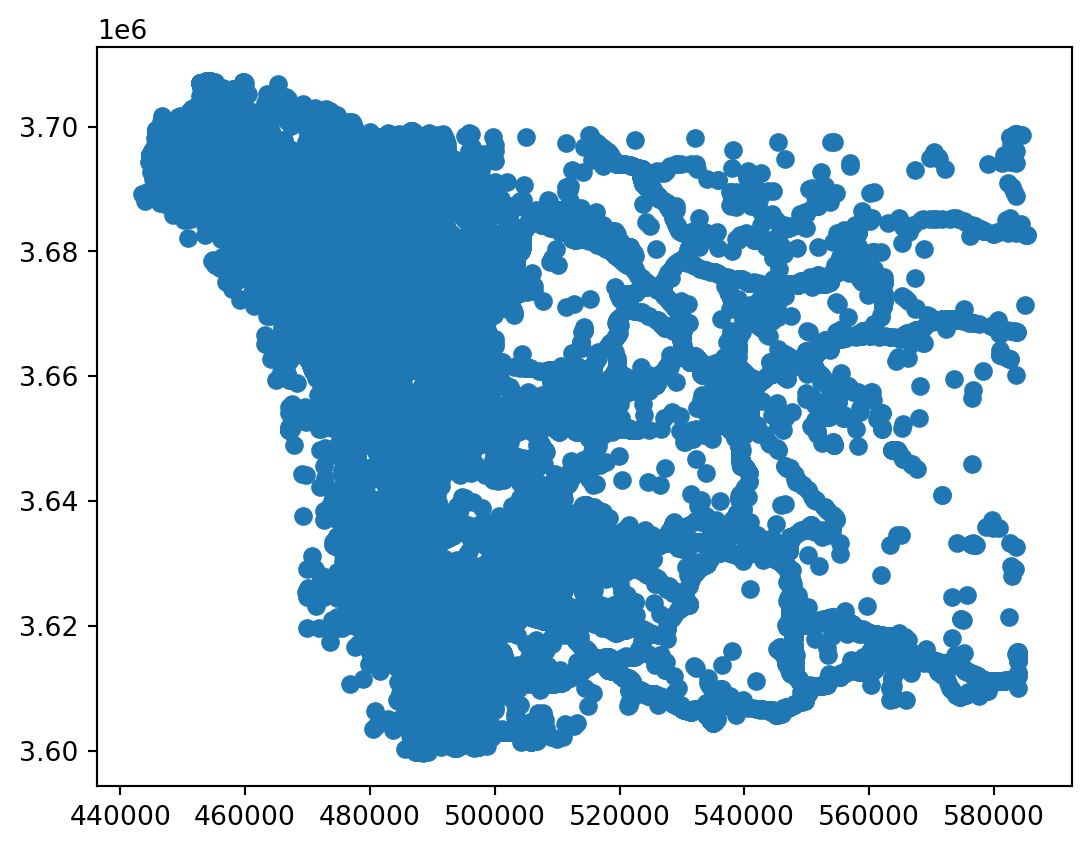
Because these points are so dense, a common way to search for “hotspots” is to plot a map using a kernel density estimator (KDE), which we can do for all events, or for subsets of events like pedestrian or bicycle collisions
# note you need statsmodels installed to run this line
ax = plot_density(sd_collisions, bandwidth=2000)
ax.axis('off')
ctx.add_basemap(ax=ax, source=ctx.providers.CartoDB.Positron, crs=sd_collisions.crs)
plt.show()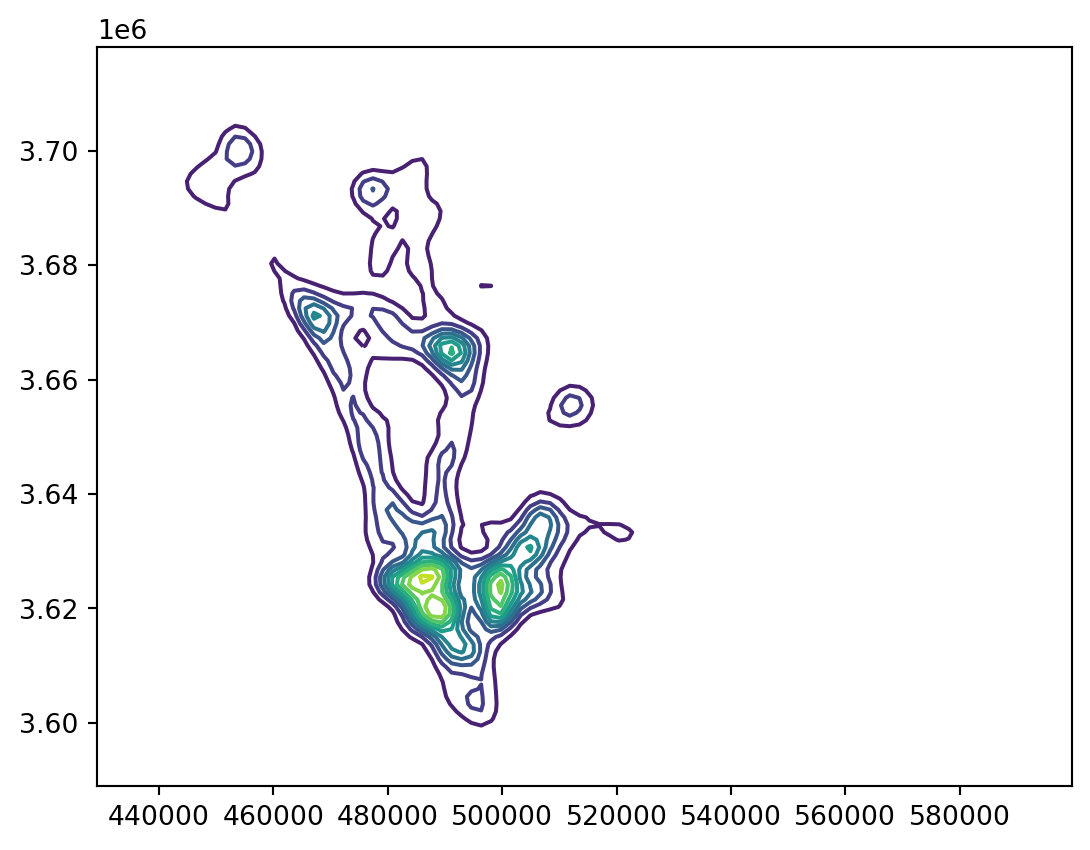
For more specificity, we can also split out pedestrian and bicycle collisions and plot the density surface of each separately.
ped_collisions = sd_collisions[sd_collisions["PEDESTRIAN_ACCIDENT"] == "Y"]
bike_collisions = sd_collisions[sd_collisions["BICYCLE_ACCIDENT"] == "Y"]

f, ax = plt.subplots(1, 2, figsize=(9, 6))

plot_density(ped_collisions, bandwidth=2000, ax=ax[0])
plot_density(bike_collisions, bandwidth=2000, ax=ax[1])
ax[0].set_title("Pedestrian Collisions")
ax[1].set_title("Bicycle Collisions")
for ax in ax:
    ctx.add_basemap(ax=ax, source=ctx.providers.CartoDB.Positron, crs=sd_collisions.crs)
    ax.axis("off")
plt.tight_layout()
plt.show()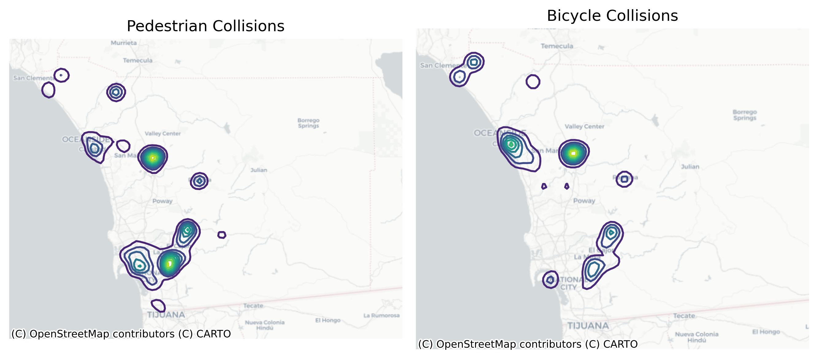
Plotting a heatmap of these points using a kernel-density estimator can give us a sense for how the events cluster in space, but it ignores the time dimension entirely. We can see that the heatmaps for pedestrian and and bicycle collisions are a little different, but it is not clear why. It could be because there are more cycle commuters in some regions of the county versus others (so more opportunities for a collision to occur) or because collision risk is higher in some places, or both. Comparisons across kernel density maps for these two classes of events is complicated because we don’t know whether they share the same population-at-risk surface underneath or risks surfaces.
The classic Knox statistic is a test for global clustering. It examines whether the pattern of spatio-temporal interaction in the events is random or not. The two critical parameters for the Knox statistic are delta and tau which define our neighborhood thresholds in space and time. The delta argument is measured in the units of the geodataframe CRS, and tau can be measured using any time measurement represented by an integer.
Here, we’ll measure time by the number of days elapsed since the start of data collection. Since the collision date is stored as a string, we can convert to a pandas datetime dtype, then take the difference from the minium date, stored in days (so our time is measured in days).
# convert to datetime
sd_collisions.COLLISION_DATE = pd.to_datetime(
    sd_collisions.COLLISION_DATE, format="%Y%m%d"
)
min_date = sd_collisions.COLLISION_DATE.min()
sd_collisions["time_in_days"] = sd_collisions.COLLISION_DATE.apply(
    lambda x: x - min_date
).dt.daysHere we set delta to 2000 and tau to 30, meaning our space-time neighborhood is looking for clusters of events that occur within one month and two kilometers of one another. To test for space-time clustering, we then instantiate a new Knox class and pass the geodataframe, the column storing values for time, and the delta and tau thresholds. Note the delta parameter is specified in units of the geodataframe coordinate system (which here is in UTM, and thus measured in meters).
ped_knox = Knox.from_dataframe(
    ped_collisions, time_col="time_in_days", delta=2000, tau=30, permutations=9999
)
Similar to the Moran classes demonstrated in the Chapter 8, the Knox classes permit two types of inferences, and provide p-values based on analytical solution, as well as a pseudo p-value that leverages computational inference; the former is the classical approach based on Kulldorff & Hjalmars (1999), and the latter is a recently-developed technique described in Rey et al. (2025) which relies on conditional permutations. To increase the precision of the latter test, you should increase the number passed to the permutations argument. The analytical p-values are stored under the p_poisson attribute.
ped_knox.p_poissonnp.float64(5.88418203051333e-15)As with other packages in the PySAL ecosystem, the computational pseudo p-values are stored under the p_sim attribute.
ped_knox.p_sim0.0001Both inferential techniques suggest significant space-time clustering at the \(\alpha=0.05\) level using these delta and tau thresholds.
Following above, we can perform the same test on bicycle collisions, asking whether we observe spatiotemporal hotspots of collisions where we have a high frequency of bicycle accidents in a defined geographic area and short period of time. If so, we will reject the null hypothesis of no interaction.
bike_knox = Knox.from_dataframe(
    bike_collisions, time_col="time_in_days", delta=2000, tau=30, permutations=9999
)bike_knox.p_poissonnp.float64(0.0)bike_knox.p_sim0.0001In both the pedestrian and bicycle collision data the p-values (for both analytical and permutation-based inference) are significant, demonstrating evidence of space-time clustering in the collisions. That is, some times and places appear to be more dangerous than others. Using a local Knox statistic, we can start investigating where and when these places might be.
As with a statistic like Moran’s \(I\), the Knox statistic can be decomposed into a local version that describes, at an observation level, whether the event at a given location and time is a member of a significant space-time cluster. This can be considered a kind of “hotspot” analysis where the locally significant values identify particular pockets of the study region (and time period) where events are clustered (Brooke Marshall et al., 2007; Piroutek et al., 2014).
ped_knox_local = KnoxLocal.from_dataframe(
    ped_collisions.set_index("CASE_ID"), time_col="time_in_days", delta=2000, tau=30
)
As a local statistic, the resulting KnoxLocal class no longer has a single \(p\)-value, but a value for each observation. Since permutations is included as a default argument in the KnoxLocal class, p-values from both the analytical and simulation-based inference are available as attributes on the fitted class
ped_knox_local.p_hypergeomarray([1. , 0.17142085, 1. , ..., 1. , 1. ,
1. ], shape=(2484,))ped_knox_local.p_simsarray([1. , 0.21, 1. , ..., 1. , 1. , 1. ], shape=(2484,))Together with the space-time neighbor relationships, we can use these p-values to identify local “hotspots”
ped_knox_local.hotspots()[["focal", "neighbor", "pvalue", "focal_time", "orientation"]]| focal | neighbor | pvalue | focal_time | orientation | |
|---|---|---|---|---|---|
| 205 | 90390796 | 90375631 | 0.36 | 2226 | lag |
| 214 | 90671972 | 8311972 | 0.20 | 2261 | lag |
| 142 | 9263257 | 9250758 | 0.04 | 3760 | lag |
| 144 | 9547792 | 9546979 | 0.02 | 4431 | lag |
| 212 | 90533779 | 8424929 | 0.01 | 2399 | lead |
| ... | ... | ... | ... | ... | ... |
| 56 | 8099893 | 8078876 | 0.06 | 2036 | lag |
| 55 | 8078876 | 8099893 | 0.03 | 2006 | lead |
| 54 | 8078797 | 8078876 | 0.20 | 1998 | lead |
| 14 | 5950645 | 5874764 | 0.01 | 702 | lag |
| 13 | 5925674 | 5901518 | 0.01 | 691 | lag |
250 rows × 5 columns
Observations are identified as hotspots if the observed number of space-time neighbors at that location exceeds the expected number. This means that every observation in the dataset is assigned a p-value that determines whether it is a significant locus of space-time interaction. From a graph theoretic perspective, the number of space-time neighbors for a unit is the number of incident edges for that node, with the graph being formed as the intersection of two other graphs: one for temporal neighbors and one for spatial neighbors. p-values for each node are determined as the probability of exceeding the number of incident edges in the space-time graph given the number of incident edges in each of the temporal and spatial graphs for that unit under the assumption of no space-time interaction.
Since we can use either computational/permutation-based inference or an analytical approximation, we can also use the analytical p-values to define hotspots
ped_knox_local.hotspots(inference="analytic")[
["focal", "neighbor", "pvalue", "focal_time", "orientation"]]| focal | neighbor | pvalue | focal_time | orientation | |
|---|---|---|---|---|---|
| 174 | 90390796 | 90375631 | 0.228722 | 2226 | lag |
| 186 | 90671972 | 8311972 | 0.102649 | 2261 | lag |
| 120 | 9547792 | 9546979 | 0.017825 | 4431 | lag |
| 182 | 90533779 | 8424929 | 0.001876 | 2399 | lead |
| 50 | 8424929 | 90533779 | 0.002090 | 2405 | lag |
| ... | ... | ... | ... | ... | ... |
| 35 | 8099893 | 8166763 | 0.041576 | 2036 | lag |
| 34 | 8078876 | 8099893 | 0.020349 | 2006 | lead |
| 33 | 8078797 | 8078876 | 0.159422 | 1998 | lead |
| 11 | 5950645 | 5874764 | 0.000168 | 702 | lag |
| 10 | 5925674 | 5901518 | 0.000417 | 691 | lag |
227 rows × 5 columns
And finally we can plot the hotspots to see where they are. By default:
crit value) shows up as grayThus, a “hotspot” is defined as the collection of points containing a “focal” observation, and its “space-time” neighbors that co-occur inside the delta and tau thresholds. In the plot, these are connected by a set of lines (comprising a small network), and the hotspot table identifies which observation is a focal observation and, if not, whether the hotspot member leads or lags the focal observation in time.
_, ax = plt.subplots(figsize=(5, 5))
ped_knox_local.plot(ax=ax).axis("off")
plt.show()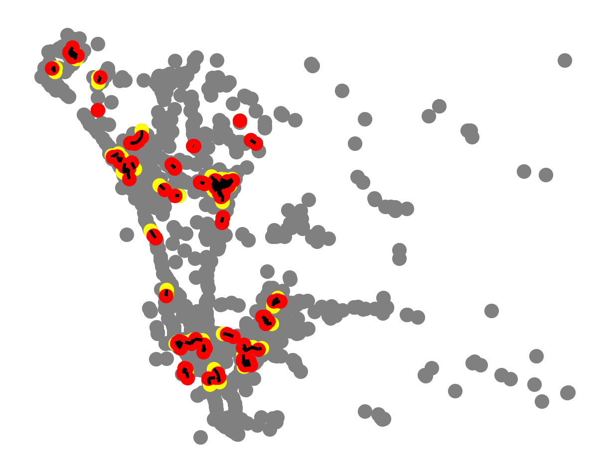
You can also customize the plot if you like
f, ax = plt.subplots(figsize=(5, 5))
ax = ped_knox_local.plot(point_kwargs={"alpha": 0.2}, plot_edges=False, ax=ax)
ctx.add_basemap(ax, source=ctx.providers.CartoDB.Positron, crs=sd_collisions.crs)
ax.axis("off")
plt.show()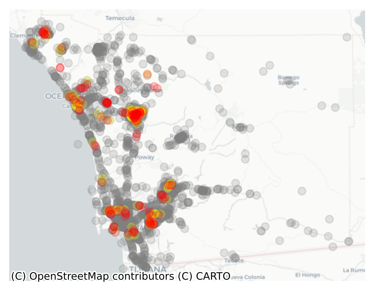
For convenience, there is also an interactive version of the hot spot map that uses the same defaults. In the interactive version, an edge (line) is drawn between members of space-time neighborhoods. This makes it easy to identify the “neighborhood” of significant events.
ped_knox_local.explore(plot_edges=True)bike_knox_local = KnoxLocal.from_dataframe(
bike_collisions, time_col="time_in_days", delta=2000, tau=30
)
bike_knox_local.explore()Comparing these maps, it looks like with these delta and tau parameters, the maps show similarities but also differences. Places like downtown, La Presa, or Escondido can be collision hotspots for both cyclists and pedestrians. But for cyclists, Coronado and Carlsbad show up as particularly dangerous locations.
Continuing with the analysis, the difference between these two hotspot locations could be because of differences in the local environment, such as poorer cycling infrastructure in Coronado and Carlsbad. But these hotspots could also just reflect that these places have greater numbers of cyclists, and thus, tend to have more frequent collisions.
These data span a long time horizon, and in this simplified demonstration, we haven’t considered the population shift bias, which occurs if the underlying spatial distribution of activities changes over time (Mack et al., 2012). In the case of vehicle collisions shown here, there is reason to believe that the underlying population at risk may have shifted over time, which could introduce a known bias into our inference. One important assumption of the Knox statistic is that population growth is constant over the geographic subareas over time, but San Diego county is a large, sprawling region and it’s possible there is more traffic activity in some parts of the region in later time periods due to uneven urban development. If so, this increase in activity will lead bias out count of observed space-time neighbors upwards. It is important to consider the performance of the Knox statistic (and its local variant) any time the underlying population surface may vary over time.