In many contexts, researchers are interested in whether some measured level of segregation is statistically different from a random process. That is, is the level of segregation we observe in place X greater than we would expect if there were no segregation at all? Sometimes that is a useful test, and the segregation package provides computational methods for conducting such a test. But it is also important to remember that the result of our inference is based on the construction of the question.
More plainly, it’s really easy to reject a silly null hypothesis; it is important that a counterfactual be plausible. In the context of residential segregation, Massey (1978) reminds us that location choice is not a random process, and that most places will surely be ‘statistically’ segregated when examined against a null hypothesis of ‘perfect integration’, or ‘evenness’, or ‘complete spatial randomness’ (depending on your disciplinary training). Unfortunately, residential segregation by race is an empirical reality in the U.S. (though it does not necessarily need to be (Ellen, 2023)), and cities will tend to be segregated through a combination of individual choice and structural constraints (Charles, 2003; Schelling, 1971).
Ideally, we want to live in a world where we do not take segregation for granted (and in the education sphere, for example, there are reasons to believe the null hypothesis of zero segregation at the classroom or school level would be appropriate), so there is good reason for single-value inferential methods to exist in theory. But this is also a good reminder that our analyses should be based on a realistic understanding of the world, and in the U.S., Massey reminds us that we should adopt what I would call a ‘cynical prior’, when we evaluate residential segregation as a statistical phenomenon.
In the context of comparative inference, our null hypotheses become plausible in a much wider variety of circumstances (Rey et al., 2021). Is New York City less segregated today than it was 20 years ago? Is New York more segregated than Los Angeles? In these cases we are not asking whether there is a behavioral proclivity to segregate (which is not a very informative question), but whether there is a stronger sorting pattern detectable in one time period or one place versus another. These are much more plausible questions (and more interesting) than “is this place segregated or not?” but they also require a more thoughtful approach to constructing a null hypothesis of “no difference.”
The segregation package provides a framework for examining whether segregation index values are statistically significant (whether a single index is far enough away from “no segregation” that it could not happen by chance, or whether two indices are different enough from one another). This framework is useful for understanding, for example:
whether the schools in a district are segregated
whether segregation in City A is greater than City B,
whether segregation at Time 2 is greater than Time 1
Depending on the segregation index being examined and the assumptions of the researcher, a variety of estimation techniques are available. This chapter walks through the assumptions and outcomes of each.
18.1 Single Value Inference
To carry out a statistical hypothesis test, we first need to define a null hypothesis represnting our expectation under the scenario of “no segregation”. In the realm of spatial statistics, this is often referred to as ‘complete spatial randomness’, which denotes no meaningful relationship between a unit of analysis and its neighbors. If we consider segregation as a phenomenon at that occurs at the person-level or household-level, then a CSR process is equivalent to the notion of ‘evenness’ in the segregation literature
For conducting single-value inference, the segregation package offer several techniques for generating random population distributions that respect the characteristics of an input dataset. This notebook walks through the assumptions and outputs of each approach
18.1.1 Complete Spatial Randomness (CSR) for Population Sorting
To get a feel for the substance of Massey’s critique, and to work out the mechanics of single-value inference, it is useful to understand what a region would look like under the condition of purely random population sorting.
evenness includes group-level variation
systematic includes unit-level variation
individual permutation includes only location variation
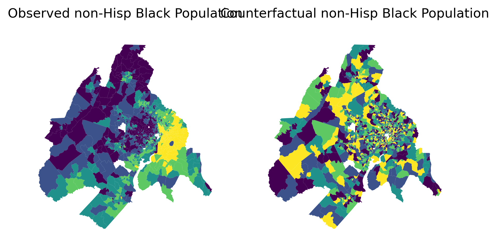
18.1.1.1 Evenness
Evenness takes draws from the population of each unit, with the probability of choosing group X equal to its regional share (locations drawing from distributions of population groups)
Code
# the regional share of nonhispanic black people in the DC region is ~25%dc.n_nonhisp_black_persons.sum() / dc.n_total_pop.sum()
np.float64(0.2515199337012678)
Code
dc[['n_total_pop']].reset_index(drop=True).head()
n_total_pop
0
6426.0
1
2076.0
2
3262.0
3
4472.0
4
5164.0
Taking 6426 draws for the tract 0 (a draw for each person), on each draw there’s a 25% chance that the chosen person is black
We haven’t changed total population in each unit or the region, but we have changed the number of group X in the region marginally
18.1.1.2 Systematic Randomization
The systematic approach takes draws from the regional population of each group, with the probability of choosing geographic unit X equal to the share of the region’s population that currently lives there (people drawing from a distribution of locations)
We haven’t changed the total number of people in any group, or changed the total population in any unit, we’ve only randomized which unit each person lives in
18.1.2 Single-Value Null Distributions
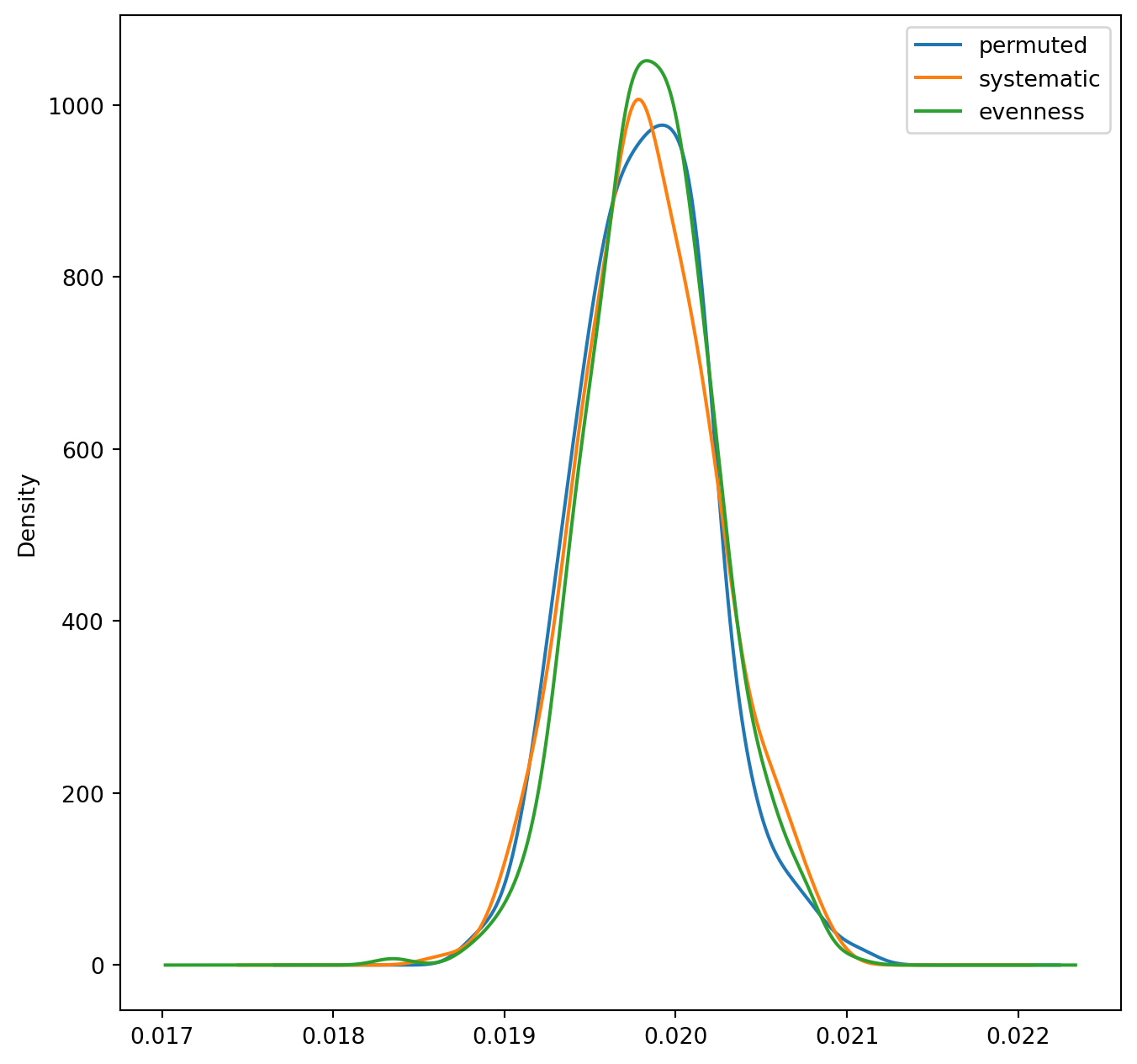
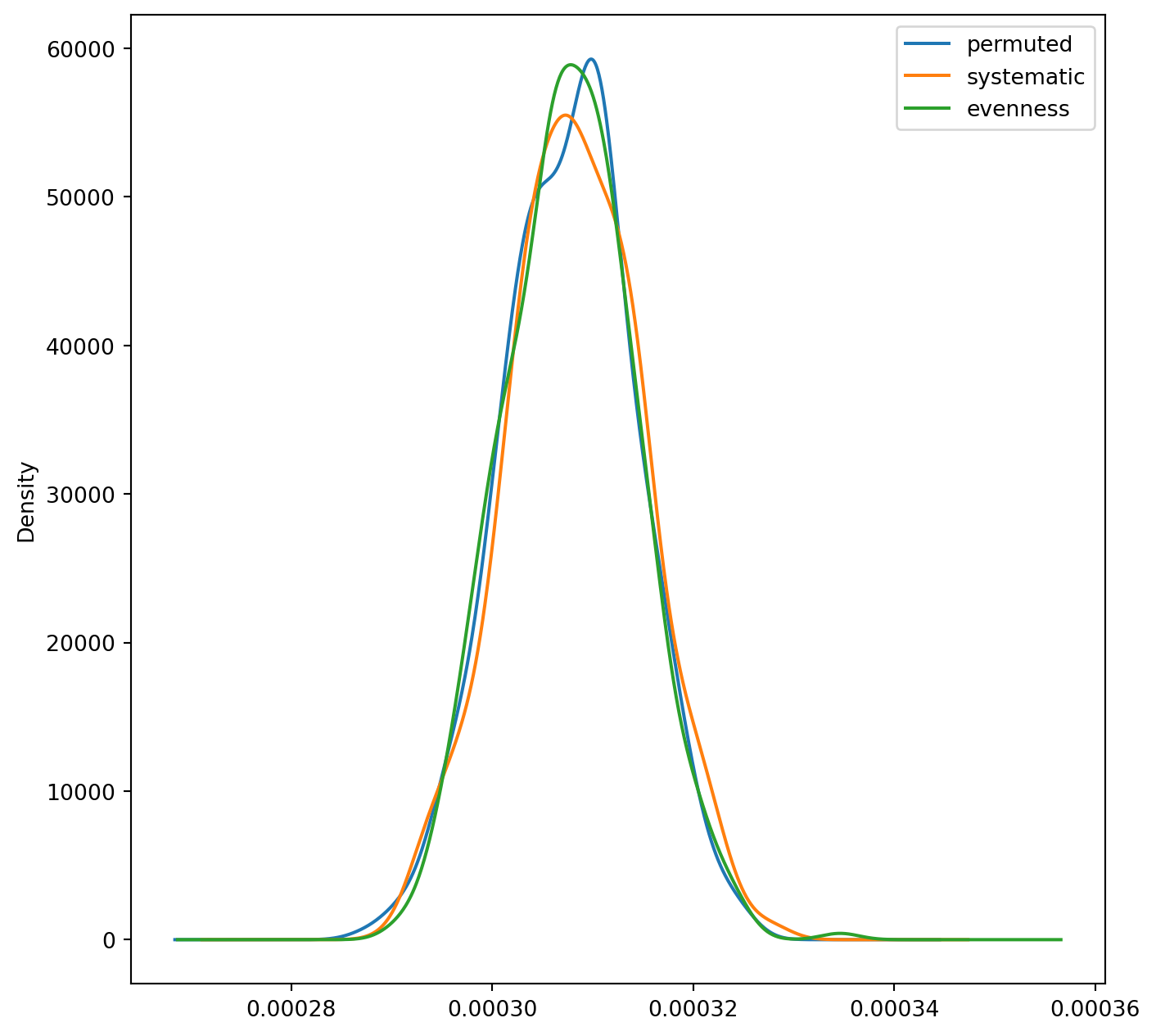
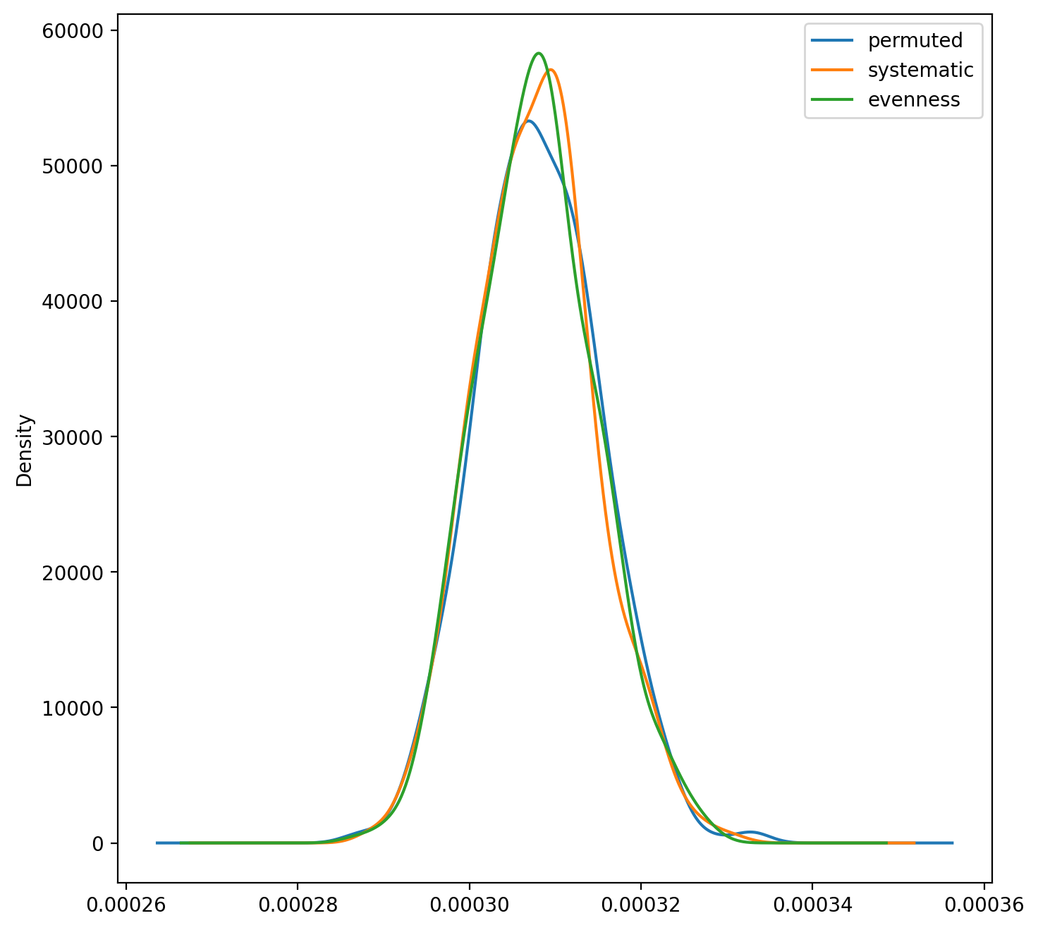
The simulate_null generates a series of simulated segregation statistics (in parallel) using the randomization functions described above. Following, those simulated values can serve as a reference distribution to test the hypothesis of “no segregation”
Code
groups = ["n_nonhisp_black_persons","n_nonhisp_white_persons","n_asian_persons","n_hispanic_persons",]G = Gini(dc, group_pop_var="n_nonhisp_black_persons", total_pop_var="n_total_pop")H = MultiInfoTheory(dc, groups=groups)
Kernel Density Estimates of Alternative (Single-group) Counterfactual Estimates
/Users/knaaptime/miniforge3/envs/urban_analysis/lib/python3.12/site-packages/joblib/externals/loky/process_executor.py:782: UserWarning: A worker stopped while some jobs were given to the executor. This can be caused by a too short worker timeout or by a memory leak.
  warnings.warn(
18.1.2.2 Multi Group
/Users/knaaptime/miniforge3/envs/urban_analysis/lib/python3.12/site-packages/joblib/externals/loky/process_executor.py:782: UserWarning: A worker stopped while some jobs were given to the executor. This can be caused by a too short worker timeout or by a memory leak.
  warnings.warn(
Kernel Density Estimates of Alternative (Multi-group) Counterfactual Estimates
Despite their different methods, all three approaches simulate similar distributions, but they differ with respect to how and in which dimensions the randomization occurs. As with Boisso et al. (1994), the distribution is not centered on zero (though it’s pretty close in the mutigroup case). In other cases, such as when minority populations are small or highly unbalanced among multiple groups, its possible that the different randomization methods could diverge to simulate different distributions
18.1.3 Inferential Methods
Code
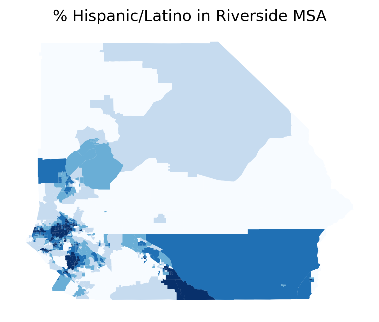
# riverside MSA in 2010rside = gio.get_census(datasets, years=[2010], msa_fips='40140')fig, ax = plt.subplots(figsize=(5,5))rside.plot('p_hispanic_persons', scheme='quantiles', cmap='Blues', ax=ax)ax.axis('off')ax.set_title('% Hispanic/Latino in Riverside MSA')plt.show()
Hispanic/Latino Population in the Riverside Metro Region
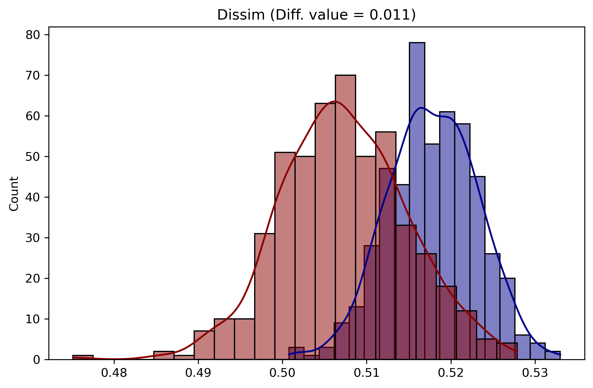
For single value inference, the segregation package tests whether the observed segregation index differs from the expected value of a segregation index under the null hypothesis of no segregation. As Boisso et al. (1994) show, the expected value of “no segregation” is not necessarily and index value of 0. The SingleValueTest class offers computational inference via a variety of methods for simulating observations under different randomization schemes
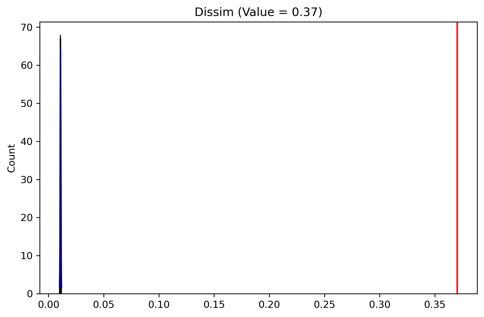
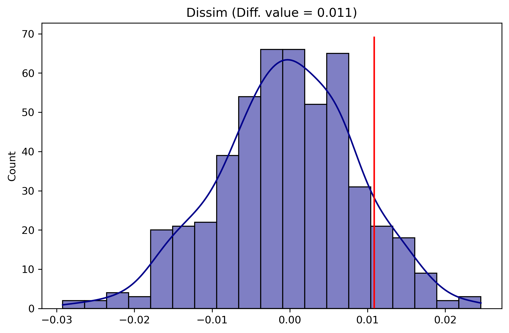
The dissimilarity statistic for riverside 2010 is 0.370
The dissimilarity index is a measure of evenness, so it is reasonable to use the evenness null approach in the SingleValueTest class. For more information on the different randomization procedures used in the single value test, have a look at the 05_simulating_random_population notebook
The p-value for the test is essentially 0. The plot method of the class will show the simulated null distribution in blue as well as the observed value for the segregation statistic in red
Code
rside_test.plot()
Code
rside_test.est_sim.mean()
np.float64(0.010847480512293754)
The est_sim attribute on the SingleValueTest class contains the segregation index values calculated for the synthetic datasets. Here we can see the estimated Dissimilarity index under the assumption of perfect evenness in Riverside is 0.011
Here the plot shows that if Riverside’s population were perfectly even across geographic units, the unequal levels in population groups would still result in a small level of Dissimilarity segregation (just barely above 0). But the distribution is nonetheless tightly distributed around that barely-zero level, whereas observed Dissimilarity in Riverside is 0.37 so we reject the null of “no segregation” in favor of the hypothesis that the Hispanic/Latino population in Riverside is significantly segregated.
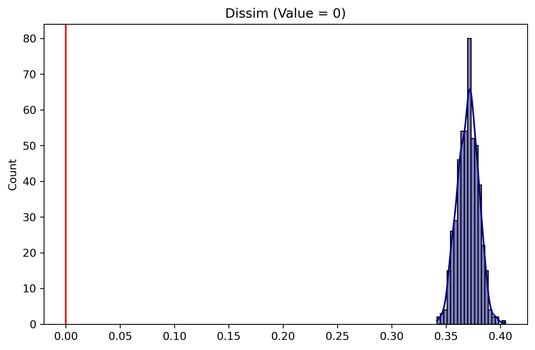
18.1.3.2 Bootstrap
As an alternative to simulating a null distribution, another resonable test for the Dissimilarity index is a bootstrap approach, used to simulate the distribution of the Dissimilarity index itself, then a given value for “no segregation” can be tested against this reference distribution. In practical terms, that means the bootstrapped index value can be tested against 0, or against the value given by a null distribution such as evenness above. This is the approach given by Allen et al. (2015)
Code
# standard test against D==0rside_test_bootstrap = SingleValueTest(D_rside, null_approach='bootstrap')rside_test_bootstrap.plot()
Plotting a SingleValueTest with the bootstrap method now shows the bootstrapped distribution of the segregation index versus the point estimate of no segregation (rather than the point estimate of the segregation index versus the simulated null distribution in the evenness approach above)
Code
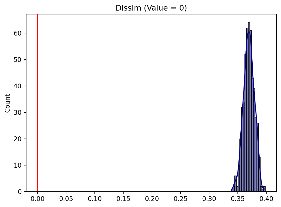
# test against the value 0.010819964855634098 estimated aboverside_test_bootstrap2 = SingleValueTest(D_rside, null_approach='bootstrap', null_value=rside_test.est_sim.mean())rside_test_bootstrap2.plot()
Whether we test against 0 or the simulated value from evenness, our inference is the same: we reject the null; Riverside is clearly segregated according to this test
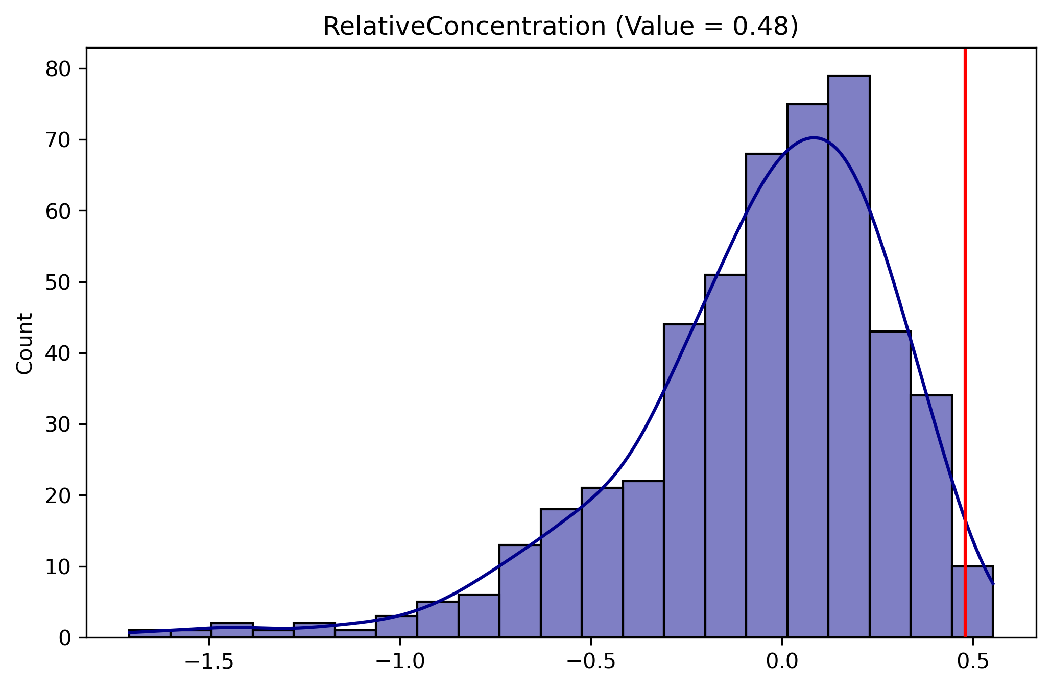
18.1.3.3 Random Geographic Permutation
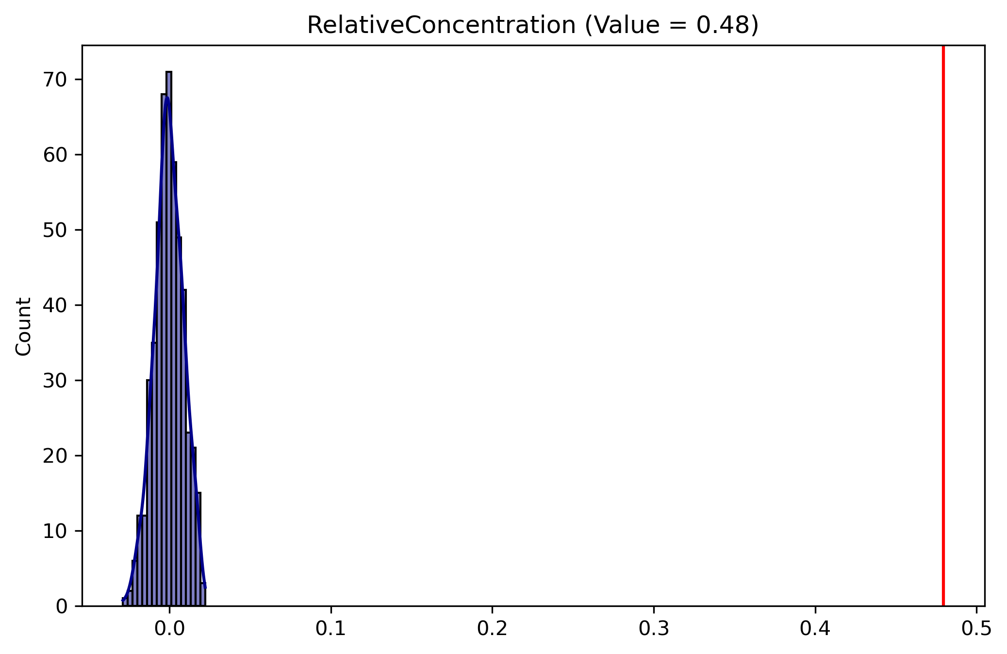
Alternatively, we might have examined a different segregation index, such as the Relative Concentration index, a spatial measure for which a different test would be appropriate
The random geographic permutation test shuffles the values of tracts in space to create a spatially-random distribution. This test leaves the total population in each group of each geographic unit, but randomizes where the unit exists in space
Code
# for spatial analysis, we need to sure rside data is in the correct projectionrside = rside.to_crs(rside.estimate_utm_crs())RCO_rside = RelativeConcentration( rside, group_pop_var="n_hispanic_persons", total_pop_var="n_total_pop")RCO_rside.statistic
It is also possible to combine the two previous approaches to first generate a simulated population under the assumption of evenness, then geographically permute the simulated data
Here the inference becomes even stronger that we reject the null
18.2 Comparative Inference
Comparative inference is particularly useful in studying residential segregation because it facilitates both temporal and spatial comparisons, allowing researchers to ask whether one place is more segregated than another, or whether a given place has become more/less segregated over time. As with single-value inference, the TwoValueTest class offers several techniques for conducting the analysis
/Users/knaaptime/miniforge3/envs/urban_analysis/lib/python3.12/site-packages/geosnap/visualize/mapping.py:171: UserWarning: `proplot` is not installed.  Falling back to matplotlib
  warn("`proplot` is not installed.  Falling back to matplotlib")
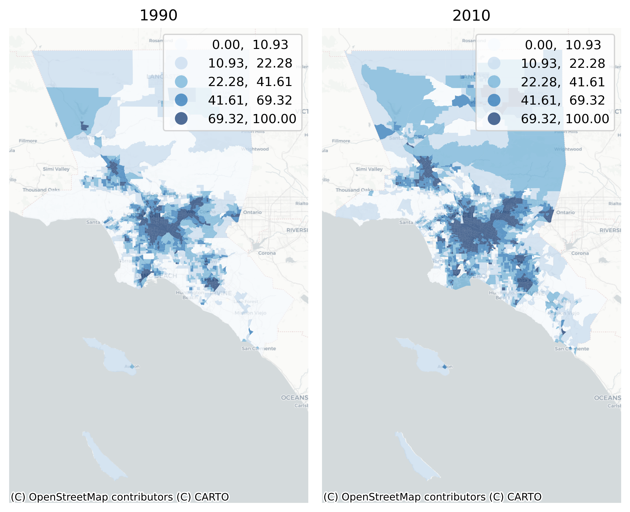
Hispanic/Latino Population in the L.A. Metro, 1990 and 2010
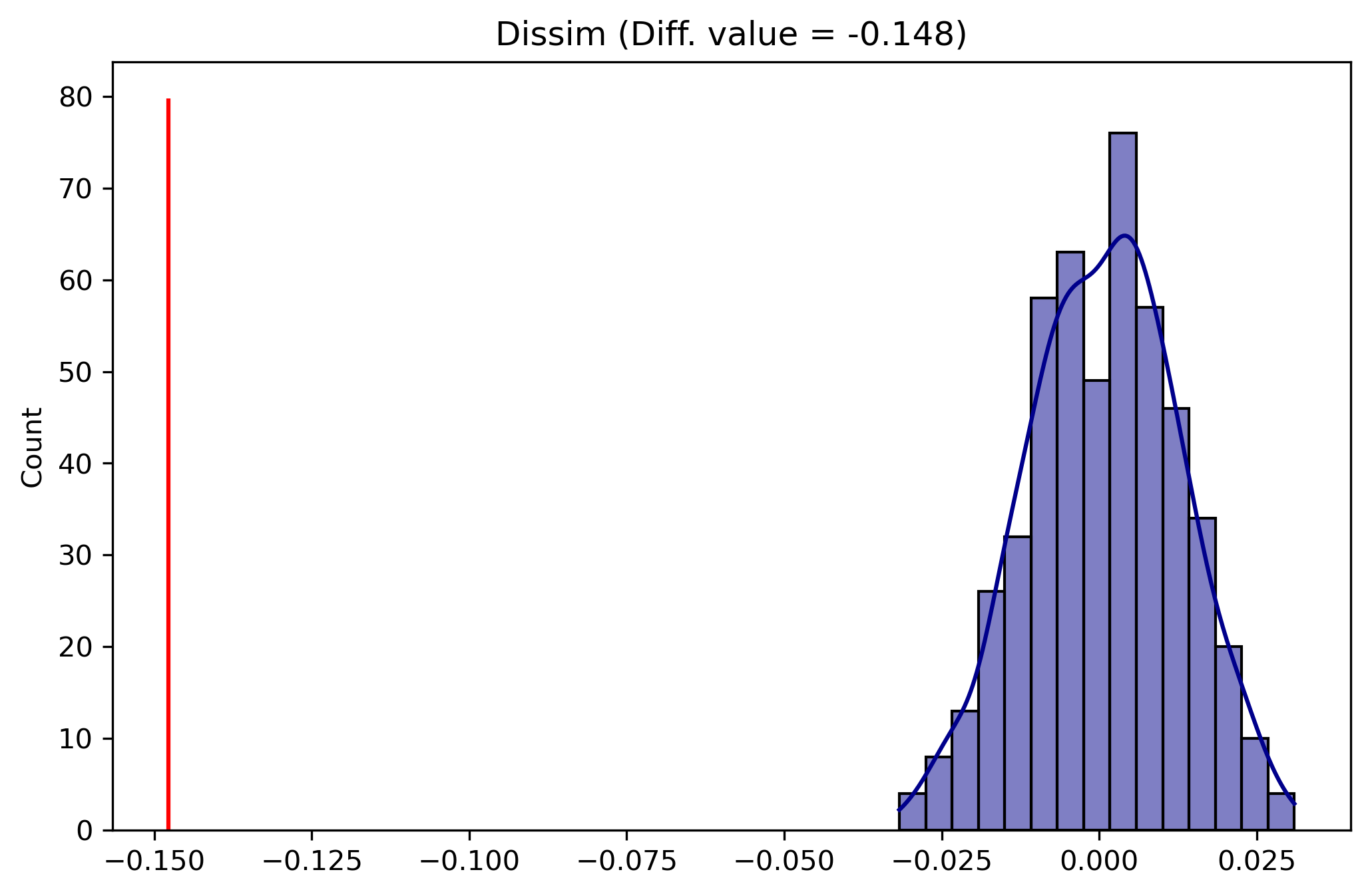
So in 20 years, Hispanic/Latino segregation in LA has increased from 0.507 to 0.518. Is that increase significantly different than a random partitioning of these data? In other words, is the difference between 1990 and 2010 large enough to be considered a ‘meaningful’ distinction, not random noise associated with these datasets? Again, there are several methods available for testing differences between segregation values. Random labelling, based on Rey & Sastré-Gutiérrez (2010) creates a set of synthetic observations by shuffling geographic units between the two cities, calculating segregation statistics on these synthetic datasets, then taking the difference between the statistics. This process results in a distribution of differences (under the null that there is no difference between the cities), and we test the observed difference against this distribution
There’s a 21.2% chance of obtaining these results at random, so we fail to reject the null hypothesis that there is no difference in segregation between the two time periods
Code
la_test_label.plot()
Plotting the class shows the distribution of simulated differences in blue as well as the estimated difference in red. Here it is clear that the observed difference falls well within the distribution
The results show that LA is significantly more segregated than Riverside, but LA is not significantly more segregated in 2010 than it was in 1990
18.2.2 Bootstrap
The bootstrap test based on Davidson (2009) uses the bootstrap resampling technique to estimate a distribution of the segregation index for each city, which provides an estimate of each index’s variance. Following, we perform a means test to see whether the mean of each distribution is significantly different from one another
Plotting a TwoValueTest class with the bootstrap method shows the bootstrapped distributions for both segregation indices. Here we can clearly see that the distributions overlap substantially
Plotting the class shows the wide berth between distributions, explaining why the p-value is so low. Again, the results show a significant difference between Riverside and LA, but not LA over time.
Allen, R., Burgess, S., Davidson, R., & Windmeijer, F. (2015). More reliable inference for the dissimilarity index of segregation. The Econometrics Journal, 18(1), 40–66. https://doi.org/10.1111/ectj.12039
Boisso, D., Hayes, K., Hirschberg, J., & Silber, J. (1994). Occupational segregation in the multidimensional case. Journal of Econometrics, 61(1), 161–171. https://doi.org/10.1016/0304-4076(94)90082-5
Ellen, I. G. (2023). A Response to David Imbroscio: Neighborhoods Matter, and Efforts to Integrate Them Are Not Futile. Housing Policy Debate, 1–4. https://doi.org/10.1080/10511482.2023.2173980
Massey, D. S. (1978). On the Measurement of Segregation as a Random Variable. American Sociological Review, 43(4), 587. https://doi.org/10.2307/2094781
Rey, S. J., & Sastré-Gutiérrez, M. L. (2010). Interregional Inequality Dynamics in Mexico. Spatial Economic Analysis, 5(3), 277–298. https://doi.org/10.1080/17421772.2010.493955