%load_ext watermark%watermark -a 'eli knaap'-v -d -u -p geopandas,geosnap
OMP: Info #276: omp_set_nested routine deprecated, please use omp_set_max_active_levels instead.
Author: eli knaap

Last updated: 2025-11-23

Python implementation: CPython
Python version       : 3.12.12
IPython version      : 9.7.0

geopandas: 1.1.1
geosnap  : 0.15.3
10.1 The ‘Egohood’ and the 20-Minute Neighborhood
As a package focused on “neighborhoods”, much of the functionality in geosnap is organized around the concept of ‘endogenous’ neighborhoods. That is, it takes a classical perspective on neighborhood formation: a ‘neighborhood’ is defined loosely by its social composition, and the dynamics of residential mobility mean that these neighborhoods can grow, shrink, or transition entirely.
But two alternative concepts of “neighborhood” are also worth considering. The first, posited by social scientists, is that each person or household can be conceptualized as residing in its own neighborhood which extends outward from the person’s household until some threshold distance (Hipp & Boessen, 2013; Kim & Hipp, 2019). This neighborhood represents the boundary inside which we might expect some social interaction to occur with one’s ‘neighbors’ (Grannis, 1998, 2005). The second is a normative concept advocated by architects, urban designers, and planners (arguably still the goal for new urbanists): that a neighborhood is a discrete pocket of infrastructure organized as a small, self-contained economic unit (Perry, 1929). A common shorthand today is the “20-minute neighborhood” (Calafiore et al., 2022).
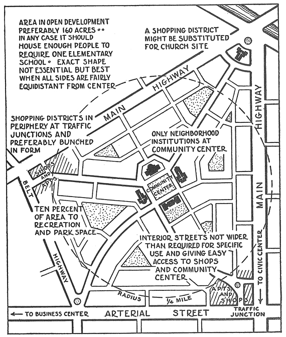
Clarence Perry’s Neighborhood Unit
The difference between these two perspectives is really what defines the origin of the neighborhood (the ‘town center’ or the person’s home), and whether ‘neighborhood’ is universal to all neighbors or unique for each resident. Both of them rely abstractly on the concept of an isochrone: the set of destinations accessible within a specified travel budget. Defining an isochrone is a network routing problem, but its spatial representation is usually given as a polygon that covers the set of locations. That polygon is also sometimes called a walkshed (or *travel shed, depending on the particular mode). For the person at the center of the isochrone, whose “neighborhood” the isochrone represents, the polygon is sometimes conceptualized as an “egohood” or “bespoke neighborhood”.
The trouble with generating isochrones is twofold. First, they are computationally intensive to create. You need to know the shortest path from an origin to all other possible destinations inside the travel threshold, and depending on the density of the network, this can scale masssively. Second, they are not straightforward to present cartographically/visually. The set of destinations reachable within the threshold is technically a set of points. If you’re constrained to a network, then we can usually assume that you also have access to potential locations between discrete destinations. For example if you’re walking along the sidewalk, you can stop at any house along the block until you reach your threshold distance. But sometimes that’s not the case. If you walk to a subway station, you can stop anywhere along the walk–until you get into the subway, then you are stuck traveling in one direction until you reach another station, then you get freedom of mobility again.
The latter case is particularly difficult to represent because it does not create a “valid” polygon… there’s a single polygon in the pre-transit zone, then the “accessible zone” collapses to a line (or nothing at all?) before opening back up into a polygon again. Like a barbell. If you take the simple route and just draw a convex hull around the accessible destinations, it will fail to collapse along the line, giving the false impression of much more ‘access’ than is realistic.
But then again, sometimes these off-network spaces are actually traversable. If two network nodes inside the travel threshold are separated by a park, then you can just walk through the park and that should be included in the visualization. If they are separated by a harbor or a mountain, you definitely can’t walk through (ok, maybe you could get through, but not without sacrificing a bit of speed at the very least).
To handle these issues, the isochrones implemented in geosnap take a straightforward approach, achieving a good balance between accuracy and speed. Specifically, we tackle the problem in two stages: first, we use pandana to generate the set nodes accessible from [a set of] destination[s]. Then we wrap an alpha shape around those destinations to create a tightly-fitted polygon. The alpha shape algorithm implemented in libpysal is also blazing fast, so the approach has worked quite well in all of our applications
Code
from folium import LayerControlfrom geosnap.analyze import isochrones_from_id, isochrones_from_gdf, pdna_to_adjfrom geosnap.io import get_acs, get_ncesfrom geosnap import DataStoreimport contextily as ctximport pandarm as pdnaimport geopandas as gpdimport pandas as pdimport osmnx as oximport matplotlib.pyplot as pltfrom geosnap import DataStorefrom geosnap.io import get_acs, get_network_from_gdffrom geosnap import analyze as gazfrom geosnap import io as giofrom routingpy import Valhallafrom shapely.geometry import Polygondatasets = DataStore()%load_ext jupyter_black
To generate a routable network, use the geosnap get_network_from_gdf function. Alternatively, you can also use pandana or urbanaccess directly. In a pinch, you can also download one of the metropolitan-scale pedestrian networks for the U.S. from geosnap’s quilt bucket, however these networks are several years old and intended primaryly for pedagogical purposes. The files are named for each CBSA fips code and extend 8km beyond the metro region’s borders to help mitigate edge effects. Here, we’ll use the quilt version from the San Diego region.
Code
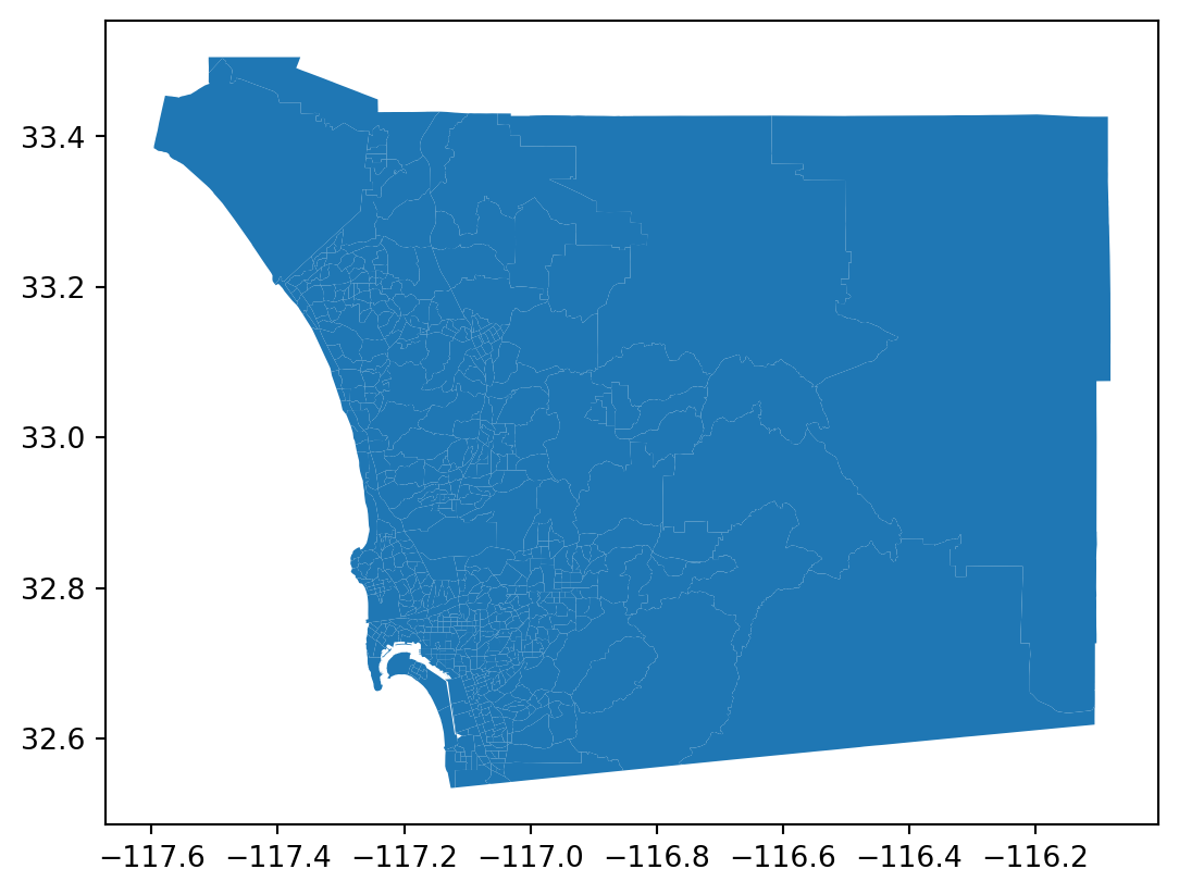
sd_tracts = get_acs(datasets, county_fips='06073', years=[2018])import osifnot os.path.exists('41740.h5'):import quilt3 as q3 b = q3.Bucket("s3://spatial-ucr") b.fetch("osm/metro_networks_8k/41740.h5", "./41740.h5")sd_network = pdna.Network.from_hdf5("41740.h5")
/Users/knaaptime/miniforge3/envs/urban_analysis/lib/python3.12/site-packages/geosnap/io/constructors.py:218: UserWarning: Currency columns unavailable at this resolution; not adjusting for inflation
  warn(
Generating contraction hierarchies with 16 threads.
Setting CH node vector of size 332554
Setting CH edge vector of size 522484
Range graph removed 143094 edges of 1044968
. 10% . 20% . 30% . 40% . 50% . 60% . 70% . 80% . 90% . 100%
To generate a travel isochrone, we have to specify an origin node on the network. For demonstration purposes, we can randomly select an origin from the network’s nodes_df dataframe (or choose a pre-selected example). To get the nodes for a specific set of origins, you can use pandana’s get_node_ids function
Code
from random import samplerandom_origin = sample(sd_network.nodes_df.index.unique().tolist(),1)[0]random_origin# for reproducibility we will select a single nodeexample_origin =1985327805
Nike, er… this study says that the average person walks about a mile in 20 minutes, so we can define the 20-minute neighborhood for a given household as the 1-mile walkshed from that house. To simplify the computation a little, we say that each house “exists” at it’s nearest intersection (this is the abstraction pandana typically uses to simplify the problem when using data from OpenStreetMap. There’s nothing prohibiting you from creating an even more realistic version with nodes for each residence, as long as you’re comfortable creating the Network)
/Users/knaaptime/miniforge3/envs/urban_analysis/lib/python3.12/site-packages/geosnap/analyze/network.py:70: UserWarning: Geometry is in a geographic CRS. Results from 'centroid' are likely incorrect. Use 'GeoSeries.to_crs()' to re-project geometries to a projected CRS before this operation.

  node_ids = network.get_node_ids(origins.centroid.x, origins.centroid.y).astype(int)
origin
destination
cost
0
060730001001
060730001001
0.000000
136
060730001001
060730001002
987.565979
197
060730001001
060730002011
1221.943970
240
060730001001
060730002022
1465.890991
280
060730001002
060730001002
0.000000
Code
iso = isochrones_from_id( example_origin, sd_network, threshold=1600) # network is expressed in metersiso.explore()
/Users/knaaptime/miniforge3/envs/urban_analysis/lib/python3.12/site-packages/geosnap/analyze/network.py:70: UserWarning: Geometry is in a geographic CRS. Results from 'centroid' are likely incorrect. Use 'GeoSeries.to_crs()' to re-project geometries to a projected CRS before this operation.

  node_ids = network.get_node_ids(origins.centroid.x, origins.centroid.y).astype(int)
Make this Notebook Trusted to load map: File -> Trust Notebook
We can also look at how the isochrone or bespoke neighborhood changes size and shape as we consider alternative travel thresholds. Because of the underlying network configuration, changing the threshold often results in some areas of the “neighborhood” changing more than others
/Users/knaaptime/miniforge3/envs/urban_analysis/lib/python3.12/site-packages/geosnap/analyze/network.py:70: UserWarning: Geometry is in a geographic CRS. Results from 'centroid' are likely incorrect. Use 'GeoSeries.to_crs()' to re-project geometries to a projected CRS before this operation.

  node_ids = network.get_node_ids(origins.centroid.x, origins.centroid.y).astype(int)
Make this Notebook Trusted to load map: File -> Trust Notebook
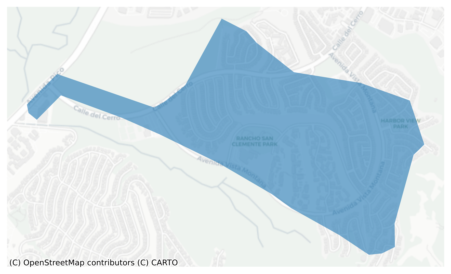
Network Isochrones with Increasing Distance Thresholds
In this example it’s easy to see how the road network topology makes it easier to travel in some directions more than others. Green space squeezes the western portion of the 1600m (20 min) isochrone into a horizontal pattern along Calle del Cerro, but the 2400m (30 minute) isochrone opens north-south tavel again along Avienda Pico, providing access to two other pockets of development, including San Clemente High School. We can also compare the network-based isochrone to the as-the-crow-flies approximation given by a euclidean buffer. If we didn’t have access to network data, this would be our best estimate of the shape and extent of the 20-minute neighborhood.
Make this Notebook Trusted to load map: File -> Trust Notebook
Code
m = planar_iso.to_crs(4326).plot(alpha=0.3)iso.plot(ax=m, alpha=0.3)example_point.plot(ax=m, markersize=4)ctx.add_basemap( ax=m, source=ctx.providers.CartoDB.Positron, crs=4326)m.axis('off')plt.show()
Network Isochrone vs. Euclidean Distance
Obviously from this depiction, network-constrained travel is very different from a euclidean approximation. That’s especially true in places with irregular networks or topography considerations (like much of California).
10.2 Isochrones for Specified Locations
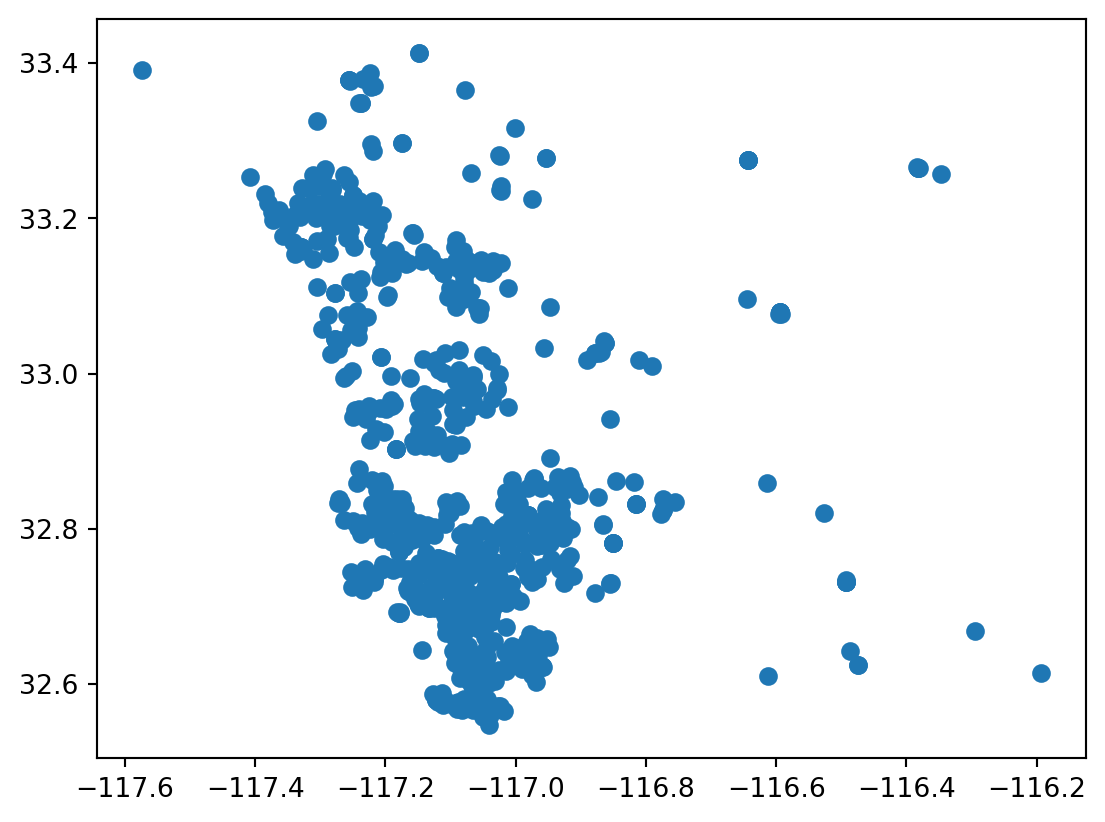
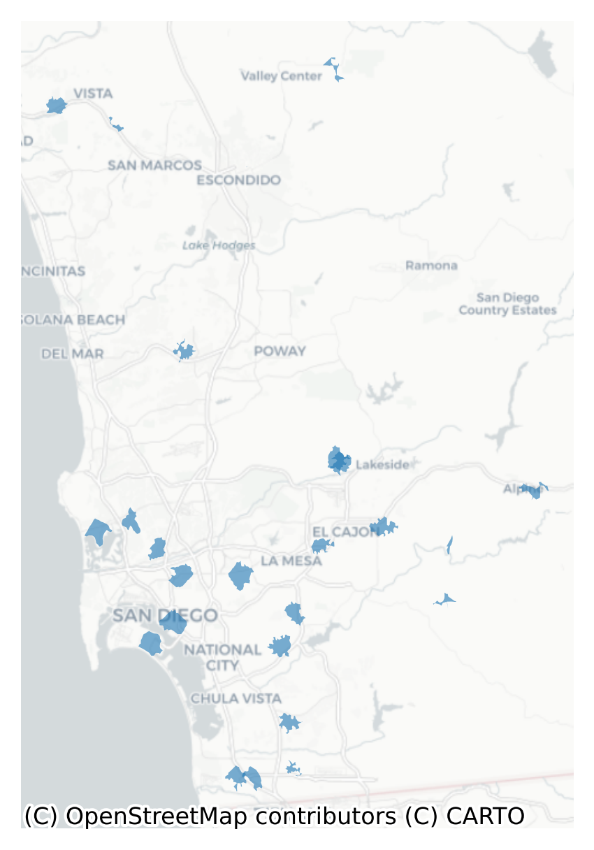
The isochrones (plural) function calculates several isochrones simultaneously, given a set of input destinations. For example we could look at the 20-minute neighborhood for schools in San Diego county.
# randomly sample 25 schools and compute their walkshedsschool_neighborhoods = isochrones_from_gdf( origins=sd_schools.sample(25), network=sd_network, threshold=1600,)school_neighborhoods.explore()
/Users/knaaptime/miniforge3/envs/urban_analysis/lib/python3.12/site-packages/geosnap/analyze/network.py:248: UserWarning: Geometry is in a geographic CRS. Results from 'centroid' are likely incorrect. Use 'GeoSeries.to_crs()' to re-project geometries to a projected CRS before this operation.

  node_ids = network.get_node_ids(origins.centroid.x, origins.centroid.y).astype(int)
/Users/knaaptime/miniforge3/envs/urban_analysis/lib/python3.12/site-packages/geosnap/analyze/network.py:70: UserWarning: Geometry is in a geographic CRS. Results from 'centroid' are likely incorrect. Use 'GeoSeries.to_crs()' to re-project geometries to a projected CRS before this operation.

  node_ids = network.get_node_ids(origins.centroid.x, origins.centroid.y).astype(int)
/Users/knaaptime/miniforge3/envs/urban_analysis/lib/python3.12/site-packages/geosnap/analyze/network.py:266: UserWarning: use_edges is True, but edge geometries are not available in the Network object. Try recreating with geosnap.io.get_network_from_gdf
  warn(
Make this Notebook Trusted to load map: File -> Trust Notebook
If we adopt the “neighborhood unit” perspective, it might be reasonable to put a school at the center of the neighborhood, as it would provide equitable access to all residents. In that case, these are your neighborhoods
10.3 Service Areas for Social Facilities
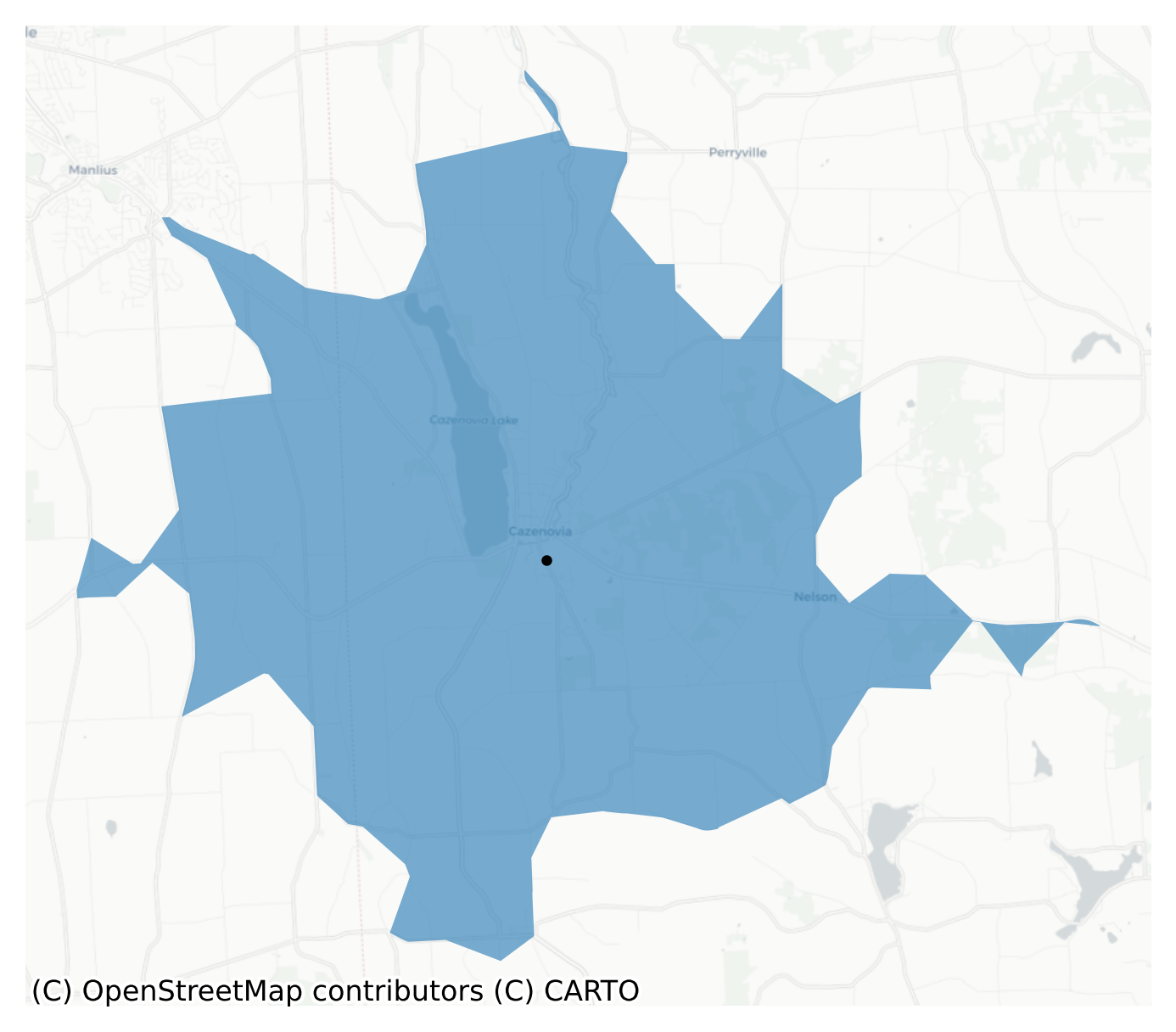
One way of thinking about isochrones is considering them as service areas. That is, given some travel budget (in time, distance, transit fare, etc), the isochrone represents the service area accessible within that budget. Imagine we were interested in the service areas around social facilities in Syracuse
Code
datasets = DataStore()# collect tracts in countytracts = get_acs(datasets, msa_fips="45060", years=[2018], level="tract")# use OSMNx to get social facilities in these tractsfacilities = ox.features.features_from_polygon( tracts.union_all(), {"amenity": "social_facility"})# keep only point geometries for illustrationfacilities = facilities[facilities.geometry.type=="Point"]# convert to a UTM projectiontracts = tracts.to_crs(tracts.estimate_utm_crs())facilities = facilities.to_crs(tracts.crs)facilities.explore(style_kwds=dict(radius=4))
Make this Notebook Trusted to load map: File -> Trust Notebook
10.3.1 Service Areas
To download a routable network from scratch using osmnx, you can use the get_network_from_gdf function from geosnap (which will get a walk network by default). These networks are more accurate for generating isochrones than the pedagogical networks stored in quilt because they include the edge geometries (e.g. the roads) that help the hull algorithm fit better.
Code
walk_net = get_network_from_gdf(tracts)
/Users/knaaptime/miniforge3/envs/urban_analysis/lib/python3.12/site-packages/geosnap/io/networkio.py:71: UserWarning: GeoDataFrame is stored in coordinate system EPSG:32618 so the pandana.Network will also be stored in this system
  warn(
Generating contraction hierarchies with 16 threads.
Setting CH node vector of size 90576
Setting CH edge vector of size 238262
Range graph removed 247732 edges of 476524
. 10% . 20% . 30% . 40% . 50% . 60% . 70% . 80% . 90% . 100%
10.3.1.1 Comparing Hull algorithms
To create the service area, we need to bound the set of reachable intersections using some kind of polygon. The resolution of the service area is dependent on the resolution of the network (i.e. since geosnap and pandana do not interpolate along the road network, greater intersection density will result in a more well-defined polygon). There are different bounding-polygon algorithms to choose from. The default is shapely’s concave_hull implementation, with the alpha_shape_auto algorithm from libpysal available as an alternative.
The alpha shape version of the concave hull is the most resource intensive because it tries to optimize the alpha parameter. This also makes it the slowest.
Code
m = alpha.explore()facilities.explore(m=m, color="black", style_kwds=dict(radius=3))
Make this Notebook Trusted to load map: File -> Trust Notebook
The concave hull algorithm in shapely does not do automatic optimization, but requires setting a ratio parameter, with smaller values resulting in tighter bounding polygons. If the ratio parameter is set too low, the bounding polygon can be too tight
Code
m = ch01.explore()facilities.explore(m=m, color="black", style_kwds=dict(radius=3))
Make this Notebook Trusted to load map: File -> Trust Notebook
Make this Notebook Trusted to load map: File -> Trust Notebook
10.3.2 Driving Service Areas
Be very careful with driving times… There are lots of edges with no speed information (requiring us to make strong assumptions), and even at best, these represent free-flow conditions. To get an automobile network, change network_type='drive' and add_travel_times=True When using travel-time based impedance, travel times are measured in seconds. See the OSMnx documentation for more details (Boeing, 2024).
Code
drive_net = get_network_from_gdf(tracts, network_type="drive", add_travel_times=True)# 10 minute drive-sheddrive_chrone = isochrones_from_gdf( facilities, network=drive_net, threshold=600, ratio=0.15, allow_holes=False)# look at only the first recordm = drive_chrone.iloc[[1]].explore()facilities.iloc[[1]].explore(m=m, color="black", style_kwds=dict(radius=6))
/Users/knaaptime/miniforge3/envs/urban_analysis/lib/python3.12/site-packages/geosnap/io/networkio.py:71: UserWarning: GeoDataFrame is stored in coordinate system EPSG:32618 so the pandana.Network will also be stored in this system
  warn(
Generating contraction hierarchies with 16 threads.
Setting CH node vector of size 24215
Setting CH edge vector of size 65013
Range graph removed 64240 edges of 130026
. 10% . 20% . 30% . 40% . 50% . 60% . 70% . 80% . 90% . 100%
Make this Notebook Trusted to load map: File -> Trust Notebook
Code
m = drive_chrone.iloc[[1]].plot(alpha=0.6)facilities.iloc[[1]].plot(ax=m, color="black", markersize=4)ctx.add_basemap(ax=m, source=ctx.providers.CartoDB.Positron, crs=tracts.crs)m.axis("off")plt.show()
Driving Time-Based Isochrone
Remember also this is directed travel. These isochrones represent the area reachable from each social service provider; they do not necesssarily represent the origins who can reach the provider within a 10 minute drive. That is, drive networks are directed (and usually asymmetric).
10.4 Comparing with Routing Servers
Here, I’ve setup an instance of the valhalla routing server on a cloud server. It’s actually pretty easy–everything is in docker, but you won’t be able to follow along unless you setup your own server and edit the URL below accordingly. Alternatively, you can try to use the public Valhalla server, but you may be rate-limited.
Often, you need routing, or travel time matrices, or isochrones for a place, but commercial or cloud-based solutions are not an option. For example if:
you have sensitive data that can’t be sent to remote servers
you have a massive dataset and end up being rate-limited (and/or hitting a paywall)
you need control over how the network is structured and parameterized (for example if you are testing different potential transit scenarios)
All of those cases require more control over the routing than web services can provide, which leaves two strong options for local computation.
/var/folders/j8/5bgcw6hs7cqcbbz48d6bsftw0000gp/T/ipykernel_53452/2815069301.py:5: UserWarning: Geometry is in a geographic CRS. Results from 'centroid' are likely incorrect. Use 'GeoSeries.to_crs()' to re-project geometries to a projected CRS before this operation.

  zip(sdsub.geometry.centroid.get_coordinates().x.tolist(), sdsub.geometry.centroid.y)
10.4.1 The Valhalla Routing Engine
One is to setup a locally-hosted open-source routing engine and query that server instead of a commercial server (as you would do with a geocoding service). This is nice because they are highly performant, but the drawbacks are:
can be a little difficult to setup and maintain, or ingest new data
can take a ton of compute/storage/memory resources, so may require your own “server”
can make the work unreproducible in many contexts, because anyone running the code also needs access to the local server. We use tailscale to share compute resources, but that adds a small layer of complexity
First we setup a connection to the Valhalla server (this one is running on a server in my research lab, but you can point this anywhere). Alternatively, you could try the public Valhalla server
Code
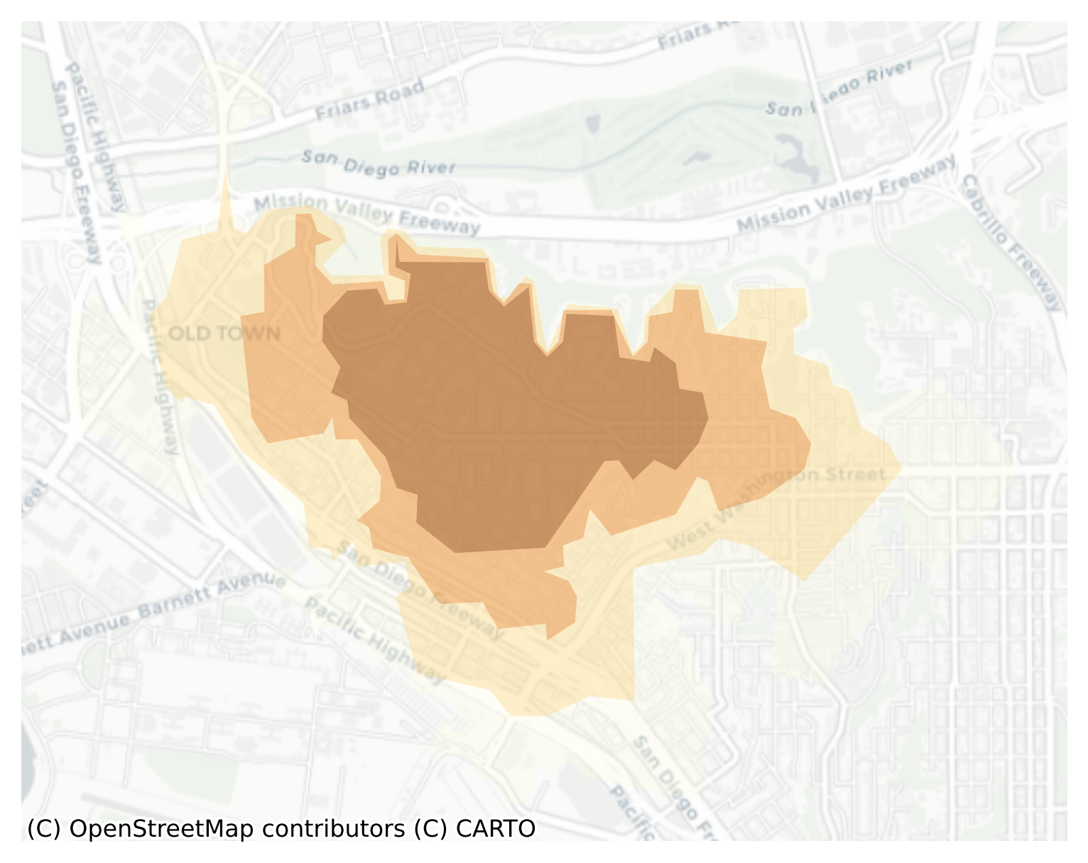
# no trailing slash, api_key is not necessary# you need to be connected to tailscale for this to workclient = Valhalla(base_url="http://cogs-research:8002", timeout=6000)# valhalla can do one origin at a time, so only pass the firsttest_isos = client.isochrones( coords[0],"pedestrian", intervals=[2500,2000,1500,1000, ], interval_type="distance",)# turn the json response into gdfsdef gdf_from_routingpy(isos): polys = [Polygon(i['geometry']['coordinates']) for i in isos.raw['features']] gdf = gpd.GeoDataFrame(geometry=polys, crs=4326)return gdfgdf = gdf_from_routingpy(test_isos)gdf["distance"] = [2500,2000,1500,1000,]gdf.explore("distance", cmap="YlOrBr_r", style_kwds={"fill_opacity": 0.3})
Make this Notebook Trusted to load map: File -> Trust Notebook
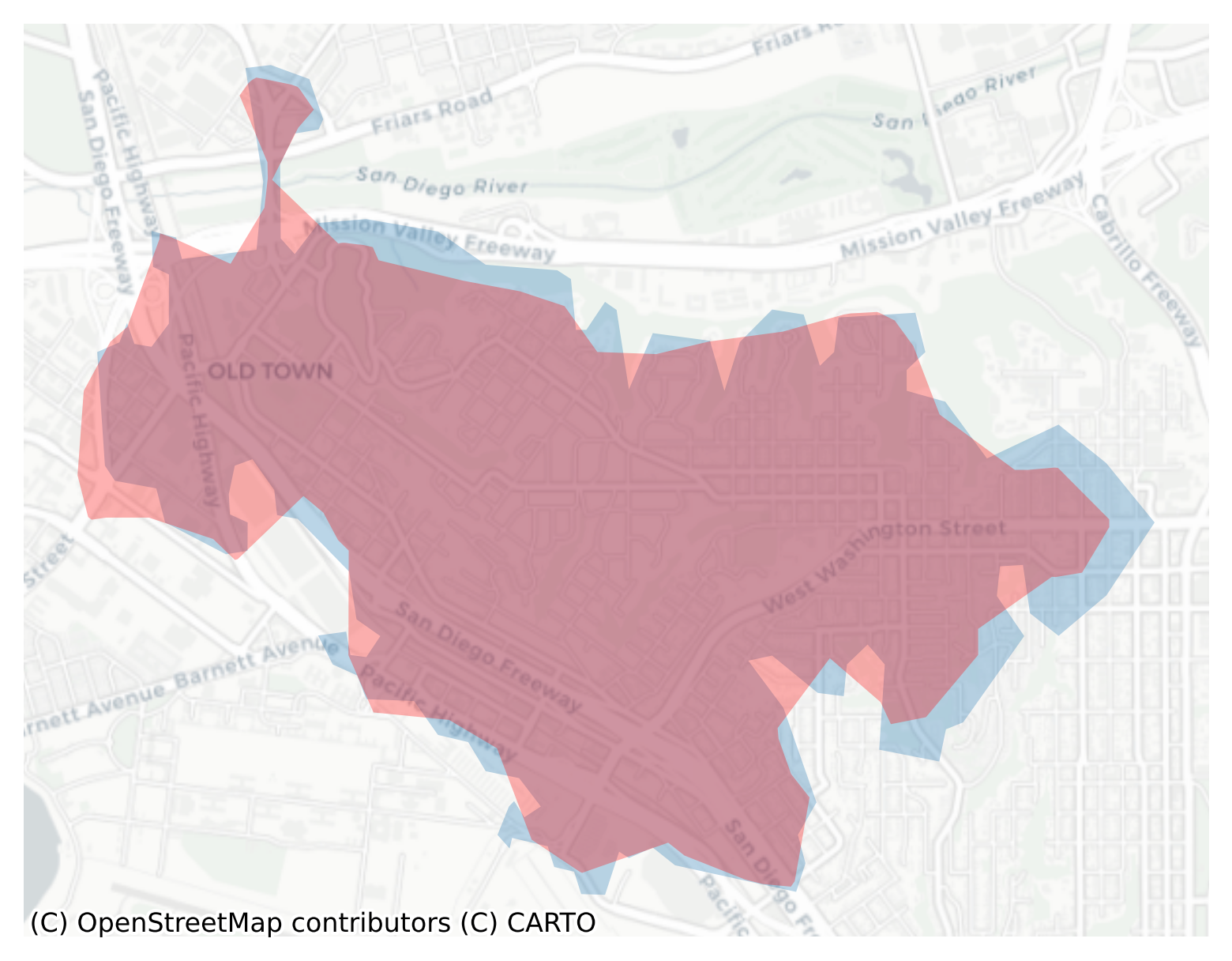
The isochrones are pretty consistent; in general, the differences between the two is that valhalla uses a tighter concave hull, which is possible because it interpolates nodes distance along the road network, rather than requiring you to hit an actual intersection (as we assume in the pandana/geosnap approach.
10.4.2.1 Comparing 2500m
Code
m = gdf.head(1).explore(name='valhalla')gisos[gisos['distance']==2500].explore(m=m, name='geosnap', color='red')LayerControl().add_to(m)m
Make this Notebook Trusted to load map: File -> Trust Notebook
Code
m = gdf.head(1).plot(alpha=0.3)gisos[gisos["distance"] ==2500].plot(ax=m, color="red", alpha=0.3)m.axis('off')ctx.add_basemap(ax=m, source=ctx.providers.CartoDB.Positron, crs=4326)plt.show()
Comparing 2.5km Isochrone from Valhalla (blue) vs Geosnap (red)
10.5 Extensions
One nice thing about this implementation is that it’s indifferent to the structure of the input network. It could be pedestrian-based (which is the most common), but you could also use urbanaccess to create a multimodal network by combining OSM and GTFS data (in the next section). For this reason, the isochrone function provided here can be much more useful than commercially-provided web services like mapbox, first because all the computation happens locally (so no paywall, and no unwanted data collection) and second because the researcher has full control over how the network is structured. This allows you to do the kinds of analyses common in actual transportation modeling and planning–like adding a new transit line, a new lane in the freeway, or a new toll road, and see how the accessibility surface responds (and how the location choices of households and businesses will reallocate given this new geography).
Running the above functions on that multimodal network would give a good sense of “baseline” accessibility in a study region. An interested researcher could then make some changes to the GTFS network, say, by increasing bus frequency along a given corridor, then create another combined network and compare results. Who would benefit from such a change, and what might be the net costs? And thus, the seeds of open and reproduciblescenario planning have been sown :)
Calafiore, A., Dunning, R., Nurse, A., & Singleton, A. (2022). The 20-minute city: An equity analysis of Liverpool City Region. Transportation Research Part D: Transport and Environment, 102, 103111. https://doi.org/10.1016/j.trd.2021.103111
Grannis, R. (1998). The Importance of Trivial Streets: Residential Streets and Residential Segregation. American Journal of Sociology, 103(6), 1530–1564. https://doi.org/10.1086/231400
Grannis, R. (2005). T-Communities: Pedestrian Street Networks and Residential Segregation in Chicago, Los Angeles, and New York. City and Community, 4(3), 295–321. https://doi.org/10.1111/j.1540-6040.2005.00118.x
Hipp, J. R., & Boessen, A. (2013). Egohoods As Waves Washing Across The City: A New Measure Of "Neighborhoods". Criminology, 51(2), 287–327. https://doi.org/10.1111/1745-9125.12006
Kim, Y.-A., & Hipp, J. R. (2019). Street Egohood: An Alternative Perspective of Measuring Neighborhood and Spatial Patterns of Crime. In Journal of Quantitative Criminology. Springer US. https://doi.org/10.1007/s10940-019-09410-3
Perry, C. (1929). The neighborhood unit, regional plan of New York and its environs. The Urban Design Reader, 78–89.