5  Areal Interpolation

“The ability of some GIS to reaggregate data from one set of areal units to another makes the modifiable areal unit problem even more important”

– Fotheringham et al. (2007, p. 29)

import contextily as ctx
import geopandas as gpd
import geoviews as gv
import hvplot.pandas
import matplotlib.pyplot as plt
import pydeck as pdk
from geosnap import DataStore
from geosnap import io as gio
from lonboard import Map, PolygonLayer, viz
from mapclassify.util import get_color_array
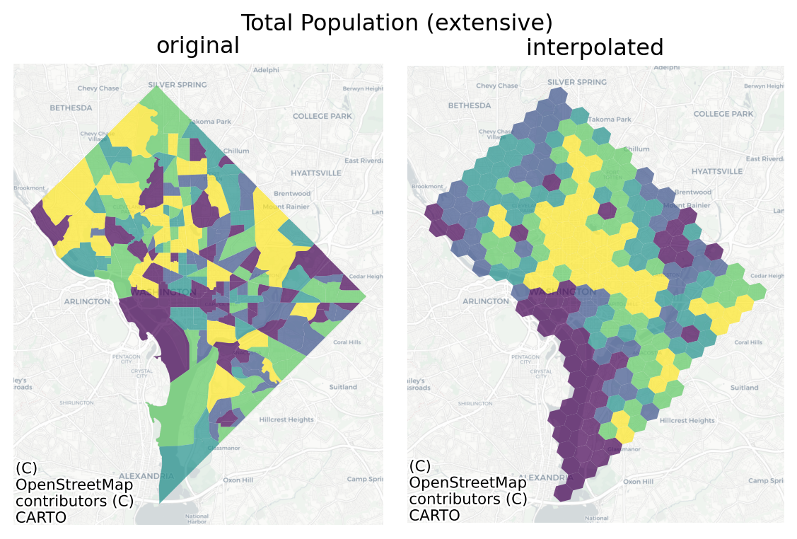
from tobler.area_weighted import area_interpolate
from tobler.dasymetric import masked_area_interpolate
from tobler.pycno import pycno_interpolate
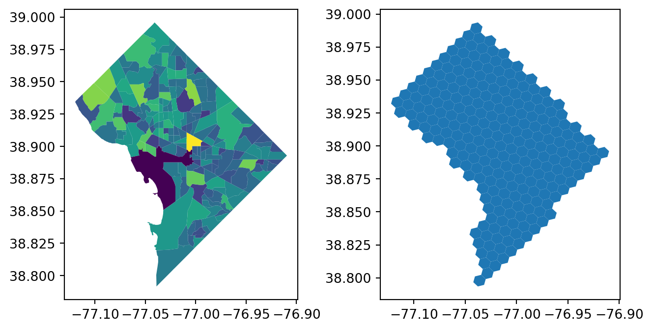
from tobler.util import h3fy

%load_ext jupyter_black
%load_ext watermark
%watermark -a 'eli knaap' -iv

/Users/knaaptime/mambaforge/envs/urban_analysis/lib/python3.12/site-packages/dask/dataframe/__init__.py:42: FutureWarning: 
Dask dataframe query planning is disabled because dask-expr is not installed.

You can install it with `pip install dask[dataframe]` or `conda install dask`.
This will raise in a future version.

  warnings.warn(msg, FutureWarning)

OMP: Info #276: omp_set_nested routine deprecated, please use omp_set_max_active_levels instead.

Author: eli knaap

matplotlib: 3.8.4
geoviews  : 1.12.0
pydeck    : 0.8.0b4
geosnap   : 0.14.0
geopandas : 0.14.4
hvplot    : 0.10.0
contextily: 1.6.1

Let’s say we want to represent the median income and total population using a regular hexgrid, but the only data available is provided at the the census-tract level. Since we can’t aggregate data upward into our new boundaries, we need some way to transfer information between the two sets of geographic units.

The tobler package provides several different ways to estimate data collected at one geography using the boundaries of a different geography.

datasets = DataStore()

dc = gio.get_acs(datasets, state_fips="11", years=[2019], level="tract")

hexes = h3fy(dc, resolution=8)

f, ax = plt.subplots(1, 2, figsize=(8, 4))

dc.plot("n_total_pop", ax=ax[0])
hexes.plot(ax=ax[1])

dc.columns

Index(['geoid', 'n_mexican_pop', 'n_cuban_pop', 'n_puerto_rican_pop',
       'n_russian_pop', 'n_italian_pop', 'n_german_pop', 'n_irish_pop',
       'n_scandaniavian_pop', 'n_foreign_born_pop',
       ...
       'p_poverty_rate', 'p_poverty_rate_over_65', 'p_poverty_rate_children',
       'p_poverty_rate_white', 'p_poverty_rate_black',
       'p_poverty_rate_hispanic', 'p_poverty_rate_native',
       'p_poverty_rate_asian', 'geometry', 'year'],
      dtype='object', length=158)

5.1 Area-Weighted Interpolation

The simplest technique available in tobler is simple areal interpolation in which variables from the source data are weighted according to the overlap between source and target polygons, then reaggregated to fit the target polygon geometries

The critical assumption in area weighted interpolation is that the variable(s) of interest is distributed uniformly across the source geometry. In practice, that is rarely true, but there are some ways to relax that assumption (in the next section).

A good way to think about this is with the figure from a classic Tobler paper on the subject. Imagine you were trying to transfer data collected at the state level, and convert it to some other meso-geography, like a PUMA or large hexgrid. The assumption we make with area-weighted interpolation is that each variable is distributed uniformly across space within each state

Population Density by State as shown in Tobler (1979)

states = datasets.states()
counties = datasets.counties()

ca_tracts = gio.get_acs(datasets, state_fips="06", years=2020, level="tract")
ca_counties = counties[counties.geoid.str.startswith("06")]

county_pop = (
    ca_tracts.assign(county=ca_tracts.geoid.str[:5])
    .groupby("county")["n_total_pop"]
    .sum()
)

ca_counties = ca_counties.merge(county_pop, left_on="geoid", right_index=True)

colors = get_color_array(ca_counties.n_total_pop, scheme="quantiles", k=8, cmap="Blues")

ca_hexes = h3fy(ca_counties, resolution=3, clip=True, buffer=True)

/Users/knaaptime/mambaforge/envs/urban_analysis/lib/python3.12/site-packages/geosnap/io/util.py:275: UserWarning: Unable to find local adjustment year for 2020. Attempting from online data
  warn(
/Users/knaaptime/mambaforge/envs/urban_analysis/lib/python3.12/site-packages/geosnap/io/constructors.py:215: UserWarning: Currency columns unavailable at this resolution; not adjusting for inflation
  warn(
/Users/knaaptime/mambaforge/envs/urban_analysis/lib/python3.12/site-packages/tobler/util/util.py:117: UserWarning: The source geodataframe is stored in a geographic CRS. Falling back to estimated UTM zone to generate desired buffer. If this produces unexpected results, reproject the input data prior to using this function
  warn(

h = PolygonLayer.from_geopandas(
    ca_hexes,
    get_fill_color=(255, 71, 76),
    get_line_color=(0, 0, 0),
    opacity=0.3,
    stroked=True,
    get_line_width=6000,
)

c = PolygonLayer.from_geopandas(
    ca_counties,
    get_elevation=ca_counties["n_total_pop"].apply(lambda x: (x**0.7)).fillna(0),
    get_fill_color=colors,
    extruded=True,
    opacity=0.6,
    wireframe=True,
)


m = Map(
    layers=[h, c],
    view_state={
        "pitch": 40,
        "bearing": 20,
        "zoom": 5,
        "latitude": ca_counties.unary_union.centroid.y - 0.1,
        "longitude": ca_counties.unary_union.centroid.x,
    },
)
m

California Population by County

That is problematic, because first, we are technically encoding both the ecological fallacy (Openshaw, 1984) and the modifiable areal unit problem (Manley, 2014) because we are literally making estimates about small areas based only on our data collected at a different resolution. And second, we know the source data is not technically uniform. Do we really think all of Texas or California or Florida have constant population density that high across the entire state? Of course not. But all we know for certain is the population density collected at the state level, so that’s the information we use to distribute information to another geographic unit. It is important to be critical about when the uniformity condition is likely to be violated badly.

Another important consideration is the difference in size between the source and target geometries.

• If source \(\gg\) target, then the interpolation operation is effectively downscaling the original information, which will induce a lot of autocorrelation (because target units falling inside a single source geometry all get assigned the same value). This is one way you can induce ‘spatial dependence’ as a consequence of measurement error (Anselin, 1988)
• if target \(\gg\) source, then the operation is effectively aggregating source polygons, in which case the estimates should be pretty accurate, but at the cost of additional information. In this case, you are throwing away variation from higher-resolution data.

results = area_interpolate(
    source_df=dc,
    target_df=hexes,
    intensive_variables=["median_household_income"],
    extensive_variables=["n_total_pop"],
)

/var/folders/79/cknfb1sx2pv16rztkpg6wzlw0000gn/T/ipykernel_53453/3633170404.py:1: UserWarning: Geometry is in a geographic CRS. Results from 'area' are likely incorrect. Use 'GeoSeries.to_crs()' to re-project geometries to a projected CRS before this operation.

  results = area_interpolate(
/Users/knaaptime/mambaforge/envs/urban_analysis/lib/python3.12/site-packages/tobler/area_weighted/area_interpolate.py:314: UserWarning: Geometry is in a geographic CRS. Results from 'area' are likely incorrect. Use 'GeoSeries.to_crs()' to re-project geometries to a projected CRS before this operation.

  den = source_df.area.values
/Users/knaaptime/mambaforge/envs/urban_analysis/lib/python3.12/site-packages/tobler/util/util.py:57: UserWarning: nan values in variable: median_household_income, replacing with 0
  warn(f"nan values in variable: {column}, replacing with 0")

fig, ax = plt.subplots(1, 2, figsize=(6, 4))

dc.to_crs(3857).plot("n_total_pop", scheme="quantiles", ax=ax[0], alpha=0.7)
results.to_crs(3857).plot("n_total_pop", scheme="quantiles", ax=ax[1], alpha=0.7)

ax[0].set_title("original")
ax[1].set_title("interpolated")
for a in ax:
    a.axis("off")
    ctx.add_basemap(ax=a, source=ctx.providers.CartoDB.Positron)

fig.suptitle("Total Population (extensive)")
plt.tight_layout()

dc.to_crs(4326).hvplot(
    c="n_total_pop",
    cmap="viridis",
    line_width=0.1,
    alpha=0.7,
    geo=True,
    tiles="CartoLight",
    xaxis=False,
    yaxis=False,
    colorbar=False,
    frame_height=500,
) + results.hvplot(
    c="n_total_pop",
    cmap="viridis",
    line_width=0.1,
    alpha=0.7,
    geo=True,
    tiles="CartoLight",
    xaxis=False,
    yaxis=False,
    colorbar=False,
    frame_height=500,
).opts(
    active_tools=["wheel_zoom"]
)

fig, ax = plt.subplots(1, 2, figsize=(8, 6))

dc.to_crs(3857).plot(
    "median_household_income", scheme="quantiles", cmap="magma", ax=ax[0]
)
results.to_crs(3857).plot(
    "median_household_income", scheme="quantiles", cmap="magma", ax=ax[1]
)

ax[0].set_title("original")
ax[1].set_title("interpolated")
for a in ax:
    a.axis("off")
    ctx.add_basemap(ax=a, source=ctx.providers.CartoDB.Positron)

fig.suptitle("Median Income (intensive)")
plt.tight_layout()

from mapclassify import Quantiles

qmi_orig = Quantiles(dc.median_household_income.dropna().values)
qmi_interp = Quantiles(results.median_household_income.values)

dc.to_crs(4326).dropna(subset="median_household_income").assign(
    label=qmi_orig.yb
).hvplot(
    c="label",
    cmap="magma",
    line_width=0.1,
    alpha=0.7,
    geo=True,
    tiles="CartoLight",
    xaxis=False,
    yaxis=False,
    colorbar=False,
    frame_height=500,
) + results.assign(
    label=qmi_interp.yb
).hvplot(
    c="label",
    cmap="magma",
    line_width=0.1,
    alpha=0.7,
    geo=True,
    tiles="CartoLight",
    xaxis=False,
    yaxis=False,
    colorbar=False,
    frame_height=500,
).opts(
    active_tools=["wheel_zoom"]
)

---

5.2 Pycnophylactic Interpolation

Pycnophylactic interpolation is based on Tobler’s method and does not distinguish between extensive and intensive variables

“Census enumerations are usually packaged in irregularly shaped geographical regions. Interior values can be interpolated for such regions, without specification of “control points,” by using an analogy to elliptical partial differential equations. A solution procedure is suggested, using finite difference methods with classical boundary conditions. In order to estimate densities, an additional nonnegativity condition is required. Smooth contour maps, which satisfy the volume preserving and nonnegstivity constraints, illustrate the method using actual geographical data. It is suggested that the procedure may be used to convert observations from one bureaucratic partitioning of a geographical area to another.”

— Tobler (1979)

Tobler’s approach does not assume a uniform distribution in the source zones but instead estimates a smooth density surface based on the centroid of the input geometries; then, it uses the source boundaries as a constraint and iteratively updates the density surface estimate to ensure that the source volume is respected (i.e. the pycnophylactic property is preserved). This can have negative consequences when the surface is poorly estimated from the input centroids

hexes = hexes.to_crs(hexes.estimate_utm_crs())

dc = dc.to_crs(dc.estimate_utm_crs())

dc_pycno = pycno_interpolate(
    source_df=dc,
    target_df=hexes,
    variables=["n_total_pop", "median_household_income"],
    cellsize=100,
    handle_null=True,
)

WARNING: nan_treatment='interpolate', however, NaN values detected post convolution. A contiguous region of NaN values, larger than the kernel size, are present in the input array. Increase the kernel size to avoid this. [astropy.convolution.convolve]
WARNING:astropy:nan_treatment='interpolate', however, NaN values detected post convolution. A contiguous region of NaN values, larger than the kernel size, are present in the input array. Increase the kernel size to avoid this.
WARNING: nan_treatment='interpolate', however, NaN values detected post convolution. A contiguous region of NaN values, larger than the kernel size, are present in the input array. Increase the kernel size to avoid this. [astropy.convolution.convolve]
WARNING:astropy:nan_treatment='interpolate', however, NaN values detected post convolution. A contiguous region of NaN values, larger than the kernel size, are present in the input array. Increase the kernel size to avoid this.

fig, ax = plt.subplots(1, 2, figsize=(10, 7))

dc_pycno.plot("n_total_pop", scheme="quantiles", ax=ax[0])
dc.plot("n_total_pop", scheme="quantiles", ax=ax[1])

ax[0].set_title("interpolated")
ax[1].set_title("original")
for ax in ax:
    ax.axis("off")
fig.suptitle("Total Population (extensive)")
plt.tight_layout()

fig, ax = plt.subplots(1, 2, figsize=(10, 7))

dc_pycno.plot("median_household_income", scheme="quantiles", cmap="magma", ax=ax[0])
dc.plot("median_household_income", scheme="quantiles", cmap="magma", ax=ax[1])

ax[0].set_title("interpolated")
ax[1].set_title("original")
for ax in ax:
    ax.axis("off")
fig.suptitle("Median Income (intensive)")
plt.tight_layout()

Open in GitHub Codespaces

:::

Anselin, L. (1988). Spatial Econometrics: Methods and Models. In Operational Regional Science Series (Vol. 4). Springer Netherlands. https://doi.org/10.1007/978-94-015-7799-1

Fotheringham, A., Brunsdon, C., & Charlton, M. (2007). Quantitative Geography. SAGE Publications Ltd. https://doi.org/10.4135/9781849209755

Manley, D. (2014). Scale, Aggregation, and the Modifiable Areal Unit Problem. In Handbook of Regional Science (pp. 1157–1171). Springer Berlin Heidelberg. https://doi.org/10.1007/978-3-642-23430-9_69

Openshaw, S. (1984). Ecological Fallacies and the Analysis of Areal Census Data. Environment and Planning A: Economy and Space, 16(1), 17–31. https://doi.org/10.1068/a160017

Tobler, W. R. (1979). Smooth pycnophylactic interpolation for geographical regions. Journal of the American Statistical Association, 74(367), 519–529. https://doi.org/10.1080/01621459.1979.10481647