Despite the wealth of valuable results, it is fair to say that the dust has not yet settled. If we want to design more effective policies for city development or redevelopment, we need a deeper understanding of the drivers behind the process of agglomeration in cities that vastly differ in size, as well as in historic and geographic attributes. Measuring the relative strength of the various types of agglomeration economies in different urban environments is one of the main challenges that spatial economics faces (Enrico, 2011; Puga, 2010).
Early models of urban spatial structure were focused almost exclusively on the monocentric model: a city with a single, large mass of jobs in the center with residential areas radiating outward (like the bid-rent model implies). For decades, however, scholars have observed cities changing form, and allowed for more complex models of urban structure, including polycentric cities with multiple nuclei of job centers. In the last section, we took an implicitly monocentric view, assuming the market center is in the geometric center of the principal city, then asking how much area this ‘employment center’ consumed. In this section we explore a method for uncovering these job centers endogenously–wherever they are in the region, and in whatever configuration they appear–then use classic measures from regional science like the Location Quotient to help characterize their composition.
The quest to find data-driven employment centers has been a methodological focus in both theoretical urban economics, which continually asks whether the monocentric model still applies, and searches for ways to allow polycentricity (Helsley & Sullivan, 1991; Redding & Rossi-Hansberg, 2017), as well as applied work in economic development, housing, land-use, and transportation planning, which ask how do such centers affect housing markets (McDonald, 1987; McDonald & McMillen, 2000), how to optimize local transport systems (and curb sprawl) (Cervero & Wu, 1998; Gordon & Richardson, 1996), and how to leverage agglomeration economies for accelerating job and wage growth (Giuliano & A. Small, 1999)–perhaps provide additional affordable housing within the commuting region (Knaap et al., 2016). Thus since the 1990s, a great deal of research has focused on methods that locate large concentrations of employment, most building from the seminal work of Giuliano & Small (1991) and subsequent additions (Giuliano et al., 2007, 2012).
We agree with McDonald (1987) that employment, not population, is the key to understanding the formation of urban centers; and that a center is best identified by finding a zone for which gross employment density exceeds that of its neighbors. We seek a definition that incorporates adjacent high density zones, and which restricts attention to centers large enough to exert a potentially significant influence.
Conventional wisdom in urban economics views employment center identification as a matter of job density (McDonald, 1987). The method developed by Giuliano & Small (1991) argues that employment centers can be defined by polygons that meet job density and total employment (jobs) threshold, which in the case of greater Los Angeles they set to ten employees per acre with a minimum of at least 10,000 total jobs. In the example below, we explore modern incantations of employment center, namely the technique developed in Knaap & Rey (2024), which depends on leveraging skills developed in the prior chapters. In this case, we build upon skills in geoprocessing, spatial graph construction, accessibility, and spatial autocorrelation, combining them for a new practical application.
15.1 Identifying Centers
An “employment center” is a large dense collection of jobs. But it is difficult and subjective to specify how large or dense a cluster of employment needs to be to comprise a “job center”. The size of a job center in Philadelphia is probably a lot larger than a center in Danville, Illinois, even if it is similarly important within its metro region. To simplify this task, we use the \(G_i\ast\) spatial statistic, which is ideal for measuring job concentrations, and moving to a statistical approach lets us use conventional relative thresholds (e.g. “one-percent significance”) rather than defining explicit cutoffs that are bespoke to a given study area.
Similar to the local Moran’s \(I\) seen in Chapter 8, the \(G_i\ast\) statistic is a measure of local spatial association that captures the similarity of values in space (Getis, 1991; Getis, 2008; Getis & Ord, 1992; Getis & Ord, 1996; Ord & Getis, 1995). Unlike the local Moran’s I which uses the mean of the spatial lag and excels at finding clusters of high and low values (i.e. hotspots and coldspots), the local \(G_i\) and \(G_i \ast\) uses the sum of the spatial lag at each location and is strong at finding large groups of positive values, and applications where coldspots are of little substantive interest. This means the \(G\) family of statistics is particularly well suited for datasets that follow a power distribution or have a natural origin at zero (e.g. percentages).
15.1.1 Start with an Accessibility Surface
This process should be familiar now after Chapter 11. First, we get the intersection IDs nearest to the centroid of each census block (mapping the job data to the travel network) and save these IDs as a variable on the input dataframe so we can use them as a join index. Then set the job variable onto the network and create an aggregation query (here, a distance-weighted sum with an exponential decay up to two kilometers).
Code
# read in datasetsdatasets = DataStore()sd_acs = gio.get_acs(datasets, county_fips="06073", years=[2021], level="tract")sd_lodes = gio.get_lodes(datasets, county_fips="06073", years="2021")sd_network = pdna.Network.from_hdf5("../data/41740.h5")sd_network.precompute(2500) # generate contraction hierarchies# get the node ids for census blockssd_lodes["node_ids"] = sd_network.get_node_ids( sd_lodes.centroid.geometry.x, sd_lodes.centroid.geometry.y)# get the node ids for tracts (for visualizationsd_acs["node_ids"] = sd_network.get_node_ids( sd_acs.centroid.geometry.x, sd_acs.centroid.geometry.y)# set the job data onto the networksd_network.set(sd_lodes.node_ids, sd_lodes.total_employees.values, name="jobs")# create an access query for 2km access with exponential decayjob_access_exp = sd_network.aggregate(2000, name="jobs", decay="exp").rename("job_access")# save the access surface back onto the blocks and tractssd_acs = sd_acs.merge(job_access_exp, left_on="node_ids", right_index=True)sd_lodes = sd_lodes.merge(job_access_exp, left_on="node_ids", right_index=True)
/Users/knaaptime/miniforge3/envs/urban_analysis/lib/python3.12/site-packages/geosnap/io/util.py:273: UserWarning: Unable to find local adjustment year for 2021. Attempting from online data
warn(
/Users/knaaptime/miniforge3/envs/urban_analysis/lib/python3.12/site-packages/geosnap/io/constructors.py:218: UserWarning: Currency columns unavailable at this resolution; not adjusting for inflation
warn(
Generating contraction hierarchies with 16 threads.
Setting CH node vector of size 332554
Setting CH edge vector of size 522484
Range graph removed 143094 edges of 1044968
. 10% . 20% . 30% . 40% . 50% . 60% . 70% . 80% . 90% . 100%
/var/folders/j8/5bgcw6hs7cqcbbz48d6bsftw0000gp/T/ipykernel_31914/3226672773.py:10: UserWarning: Geometry is in a geographic CRS. Results from 'centroid' are likely incorrect. Use 'GeoSeries.to_crs()' to re-project geometries to a projected CRS before this operation.
sd_lodes.centroid.geometry.x, sd_lodes.centroid.geometry.y
/var/folders/j8/5bgcw6hs7cqcbbz48d6bsftw0000gp/T/ipykernel_31914/3226672773.py:14: UserWarning: Geometry is in a geographic CRS. Results from 'centroid' are likely incorrect. Use 'GeoSeries.to_crs()' to re-project geometries to a projected CRS before this operation.
sd_acs.centroid.geometry.x, sd_acs.centroid.geometry.y
Removed 12657 rows because they contain missing values
This is the dataset we will now use to generate our \(G_i\ast\) statistics, and since the access variable is essentially a density surface, this means the method is effectively searching for statistically significant pockets of job density–or, spatial job clusters, exactly what we’re trying to find.
15.1.2 A Coarse Approach
As a first pass, we could simply use polygons and contiguity relationships looking for clusters of adjacent polygons which together have a significant sum of jobs. This is what many of the early papers do, though our results are beholden to the irregular size and shape of the input geometries (traditionally Traffic Analysis Zones, TAZs). Still we are forced to make subjective decisions about what counts as “large” or “important”, however we can make these decisions uniformly with the expectation that they should work reasonably in most places. To mark a job center as “large enough” we say that it falls in the top 20% of the number of jobs available, and to mark it as “dense enough”, we say that the cluster has a significant \(G_i\ast\) value at the .05% level.
Code
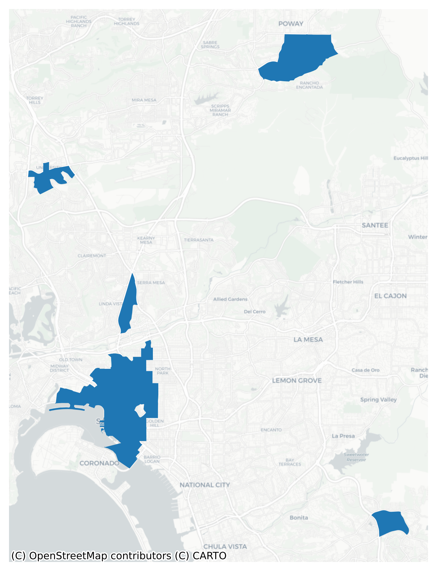
# create a Rook contiguity graph and allow units to be own-neighborswacs = Graph.build_contiguity(sd_acs, rook=False).assign_self_weight(1)# compute a local G_i\astg_jobs = G_Local(sd_acs.job_access.values, wacs, star=True)# create a new dataframe to hold the employment center datacenters = sd_acs[["geoid", "job_access", "geometry"]].copy()# assign the local p-values as a column on the dataframecenters["pvalue"] = g_jobs.p_sim# create a column of percentile rank by jobs availablecenters["job_rank"] = centers.job_access.rank(pct=True)# define subcenter as: total job access in top quintile, significant (G_i*) spatial clustersubcenters = centers[(centers.pvalue <0.05) & (centers.job_rank >0.8)]subcenters.explore(tiles="CartoDB Positron")
Make this Notebook Trusted to load map: File -> Trust Notebook
Once we have a set of local \(G_i\ast\) values and percentile ranks, we select all the polygons that meet both criteria, then use a spatial weights matrix (Graph) to dissolve contiguous polygons into centers (McMillen, 2003).
Code
# create a new Rook graph on the subsetted polygonsw_subcent = Graph.build_contiguity(subcenters, rook=False)# assign a 'center ID' column using each unique component of the Graphsubcenters["center"] = w_subcent.component_labelssubcenters["center"] = subcenters["center"].apply(lambda x: f"center {x}")# use the center ID to dissolve contiguous polyssubcenters = subcenters.dissolve("center")subcenters.explore(tiles="CartoDB Positron")
/Users/knaaptime/miniforge3/envs/urban_analysis/lib/python3.12/site-packages/geopandas/geodataframe.py:1968: SettingWithCopyWarning:
A value is trying to be set on a copy of a slice from a DataFrame.
Try using .loc[row_indexer,col_indexer] = value instead
See the caveats in the documentation: https://pandas.pydata.org/pandas-docs/stable/user_guide/indexing.html#returning-a-view-versus-a-copy
super().__setitem__(key, value)
Make this Notebook Trusted to load map: File -> Trust Notebook
Since we’re operating on census tracts, our resulting subcenters are a function of tract size and contiguity, but the data are actually much higher resolution than that. We have computed accessibility at the intersection level, rather than the tract level, so we could instead look for significant \(G_i\ast\) clusters of these intersections instead (then wrap a polygon around them). With the libpysal Graph, we can also use network distances to create our weights object, rather than relying on contiguity between polygons. This is the approach taken in Knaap & Rey (2024). Notably, this method also meets all the criteria specified by Duranton & Overman (2005) for good techniques that identify local agglomeration economies, providing evidence of “clustering of production beyond what can be explained by chance or comparative advantage” (Puga, 2010): statistical significance, avoidance of MAUP, and sensitivity to local/industrial conditions.
/var/folders/j8/5bgcw6hs7cqcbbz48d6bsftw0000gp/T/ipykernel_31914/2298782041.py:5: UserWarning: CRS mismatch between the CRS of left geometries and the CRS of right geometries.
Use `to_crs()` to reproject one of the input geometries to match the CRS of the other.
Left CRS: EPSG:4326
Right CRS: EPSG:4269
all_intersections = gpd.overlay(
The all_intersections dataframe represents job accessibility for every single intersection in the San Diego metropolitan region, which is probably a bit more detailed than we need. Just how large are we talking?
Code
all_intersections.shape
(245061, 2)
About 245 thousand nodes. That’s a really big problem, so let’s simplify and use the subset of nodes where blocks are attached.
Code
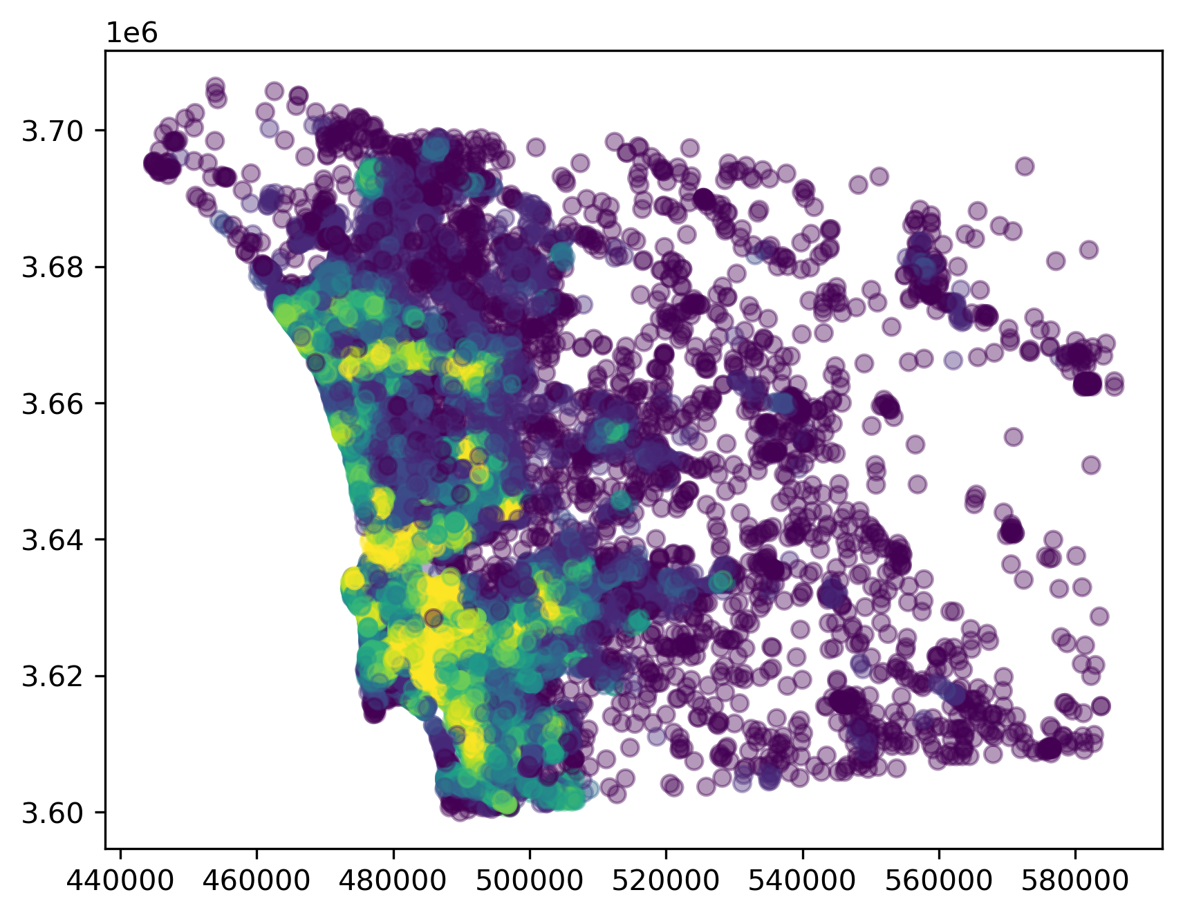
sd_lodes = sd_lodes.to_crs(sd_lodes.estimate_utm_crs())all_intersections = all_intersections.to_crs(all_intersections.estimate_utm_crs())# only the nodes attached to a census blocklodes_nodes = all_intersections[all_intersections.index.isin(sd_lodes.node_ids)]lodes_nodes.plot("job_access", scheme="quantiles", k=10, alpha=0.4)plt.show()
San Diego Intersections with Job Data
This is still extremely detailed, but we are not including additional geometries where we have no actual data points (i.e. our resolution is only as fine as the block-level where the jobs data come from). Now we use the nodes_in_range function to return an adjacency list of nodes within two kilometers and convert that into a libpysal.Graph
Code
w_dist = sd_network.nodes_in_range(lodes_nodes.index.unique(), 2000)g = Graph.from_adjacency(w_dist, "source", "destination", "distance")# ignore distance for now and treat distance-band as discrete within threshold (then row-standardize)g = g.transform("b").assign_self_weight(1)
The object g is a PySAL graph object that encodes observations as neighbors if they are within a 2km shortest-path distance along the travel network. Now we repeat the same \(G_i\ast\) analysis we used on the census polygons above, selecting the nodes that belong to significant clusters in the top 80% of job accessibility.
/Users/knaaptime/miniforge3/envs/urban_analysis/lib/python3.12/site-packages/geopandas/geodataframe.py:1968: SettingWithCopyWarning:
A value is trying to be set on a copy of a slice from a DataFrame.
Try using .loc[row_indexer,col_indexer] = value instead
See the caveats in the documentation: https://pandas.pydata.org/pandas-docs/stable/user_guide/indexing.html#returning-a-view-versus-a-copy
super().__setitem__(key, value)
Make this Notebook Trusted to load map: File -> Trust Notebook
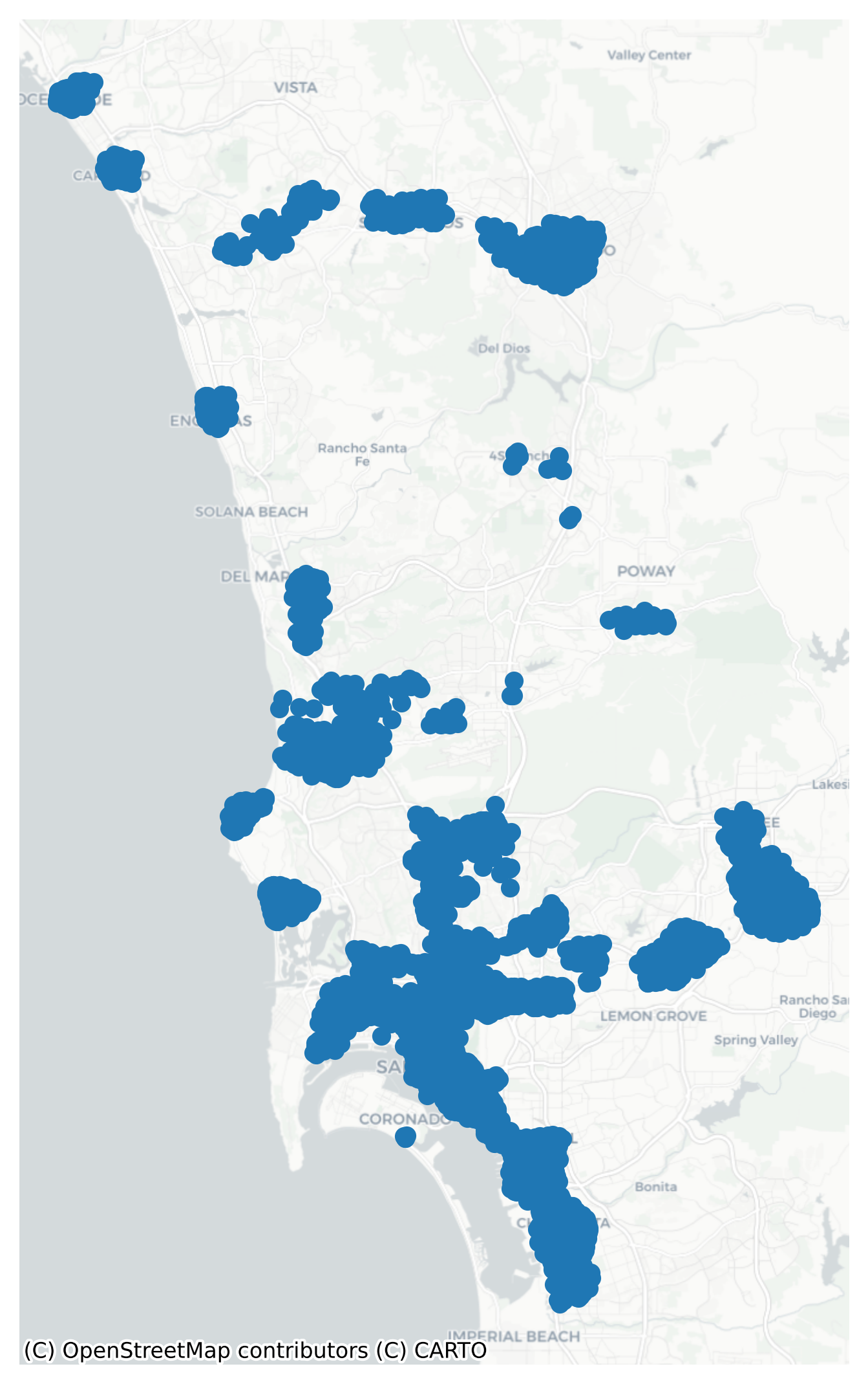
Moving to the intersection scale results in a much larger employment center footprint, because there are many more observations, the surface is much more distinct, and its easier to pick out spatial outliers. The difficulty is that now our dataset is represented as a collection of points, when we want to identify discrete center polygons.
To do that, we first define a range wherein points are considered to belong to the same center (instead of setting this with a discrete threshold rule, you could alternatively use something like DBscan). Then, for each set of points, we wrap a tightly-fitted polygon that represents the “center”. Here, we will say nodes belong to the same center if they fall within two kilometers of one another (the same threshold we used in our \(G_i\ast\)), and plot them below.
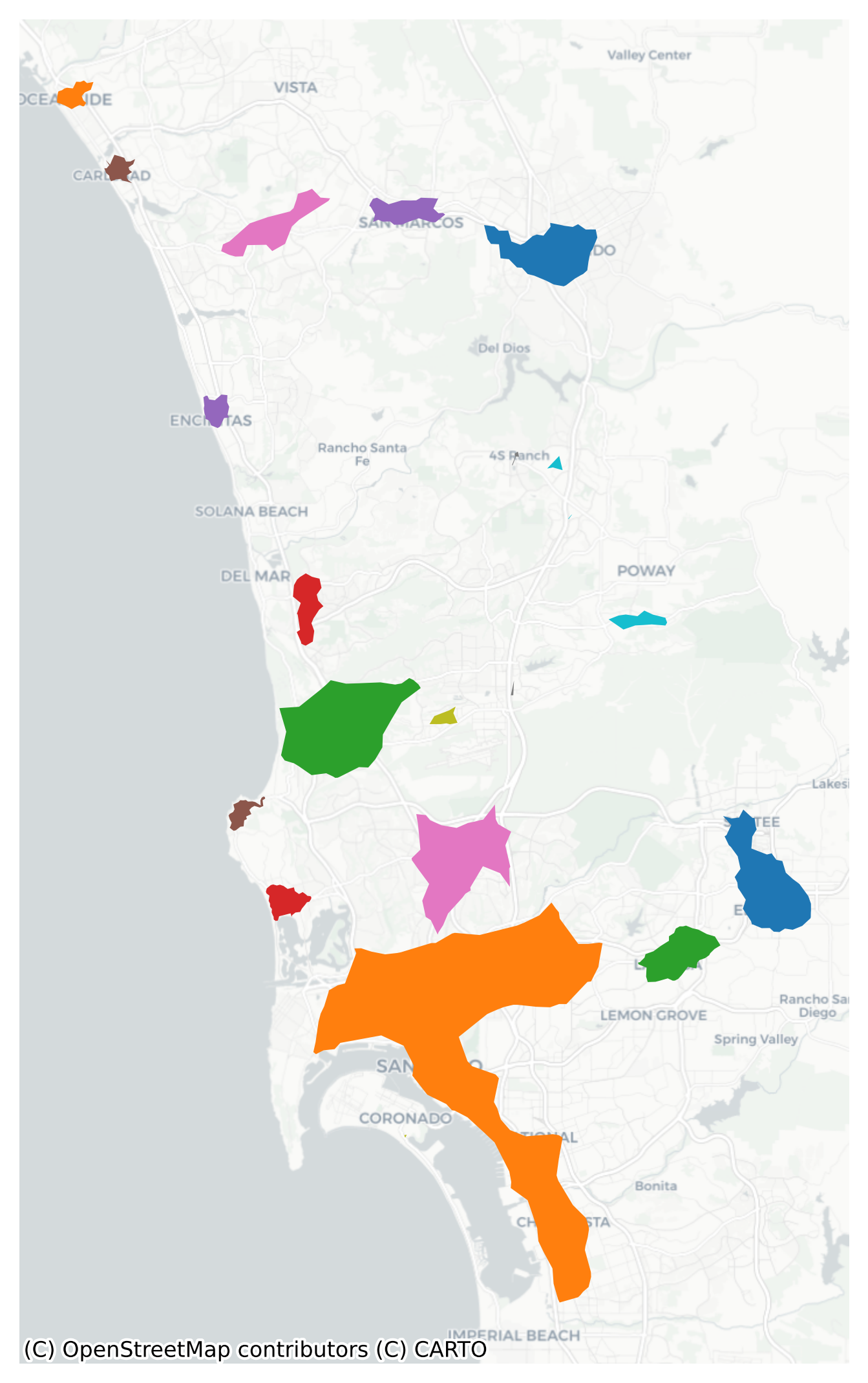
Each group of colored nodes in the map above represents a distinct job center in the San Diego region. Compared to the polygon-based analysis above, we have revealed many more employment centers (21 in total), many of which have a relatively small spatial footprint. This difference helps show the additional power we gain when moving to the finer resolution because our densities are not based on polygons that vary in size.
Code
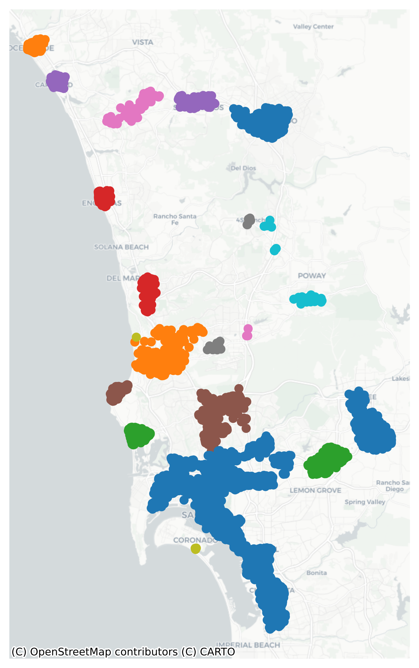
# us the alpha shapeshapes = [ alpha_shape_auto( center_nodes[center_nodes.center == i] .geometry.get_coordinates()[["x", "y"]] .values )for i in center_nodes.center.unique()]node_subcenters = gpd.GeoDataFrame(geometry=shapes, crs=center_nodes.crs)node_subcenters.reset_index()# if some centers can become degenerate polygons if they have only a single node# or if they have two nodes and become a line, so we remove any 'center' with no areanode_subcenters = node_subcenters[~node_subcenters.geometry.is_empty]node_subcenters.reset_index().explore("index", categorical=True, tiles="CartoDB Positron")
Make this Notebook Trusted to load map: File -> Trust Notebook
As a quick indicator of the method’s performance we can compute the share of the region’s employment in each center. To make things simple four ourselves, we will encode all employment outside employment centers as -999, which allows us to use a quick groupby operation, and creates an additional category for comparison.
Code
# attach center IDs to the original LODES datasd_lodes = sd_lodes.merge( center_nodes[["center"]], left_on="node_ids", right_index=True, how="left")# fill non-center nodes with dummy IDsd_lodes["center"] = sd_lodes["center"].fillna(-999)# compute the share of jobs in each industrysd_lodes.drop(columns=["geometry"]).groupby("center").sum()[ ["total_employees"]] / sd_lodes.total_employees.sum()
total_employees
center
-999.0
0.438150
0.0
0.026398
1.0
0.025300
2.0
0.189283
3.0
0.004131
4.0
0.100236
5.0
0.013516
6.0
0.005252
7.0
0.014434
8.0
0.005191
9.0
0.010920
10.0
0.004578
11.0
0.005404
12.0
0.091807
13.0
0.021969
14.0
0.002853
15.0
0.000486
16.0
0.007386
17.0
0.004442
18.0
0.000238
19.0
0.005667
20.0
0.014224
21.0
0.008137
While none of the individual centers are dramatically large–although center 2 (downtown) has ~19% of the region’s employment and center 4 (UCSD) has 10%–the dummy category representing non-center employment is only 44%. This means the remaining 56% of employment in the region is concentrated into these 21 centers which comprise an extremely small fraction of the metro’s land area.
15.1.3.1 Alternative Polygons
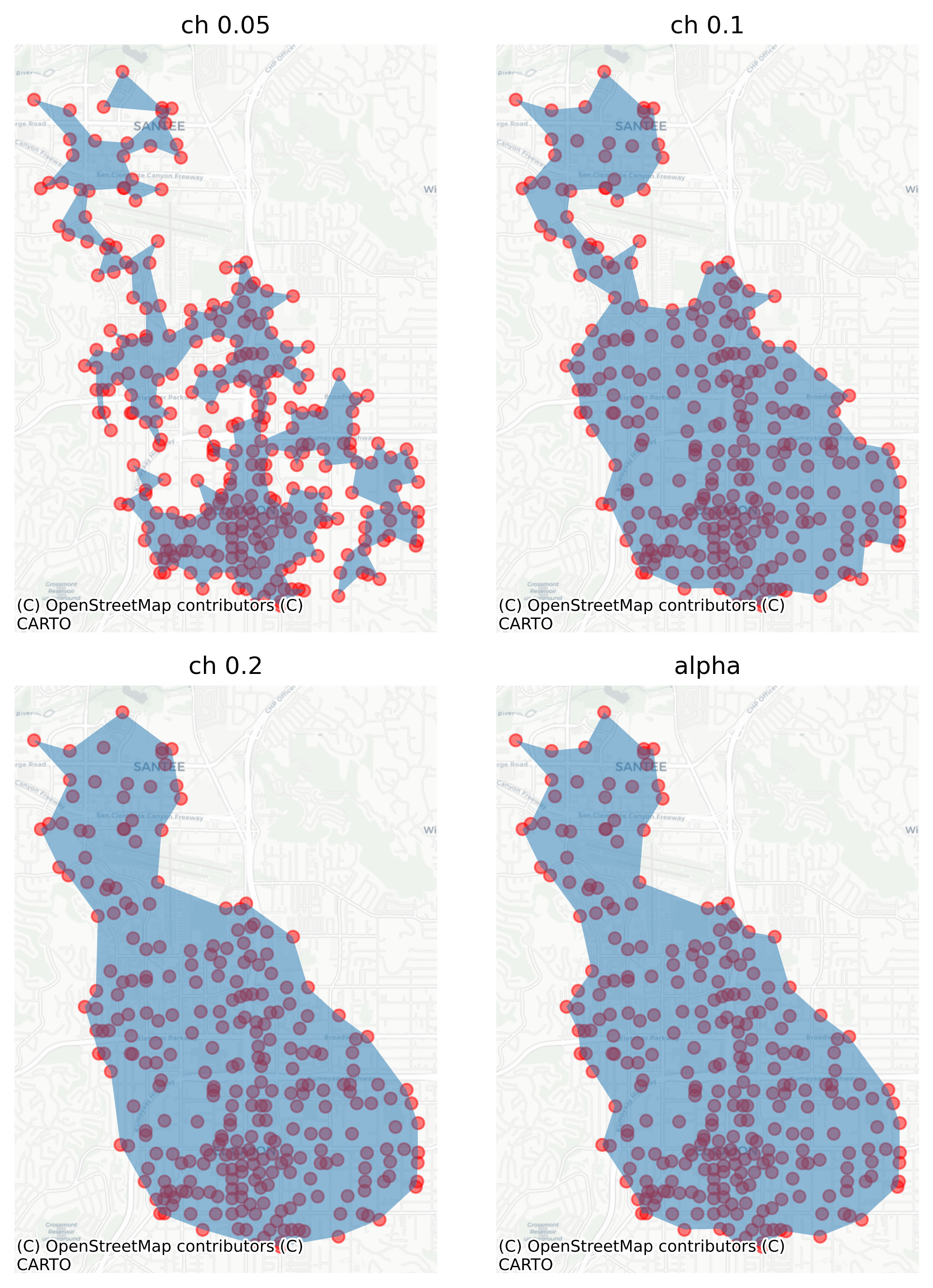
Rather than an alpha_shape, we could use other concave hull methods, e.g. from shapely. To see the effect of choosing to bound centers using different polygonization parameters, we can look at center one; these are the points belonging to it.
Similar to the isochrones in Chapter 10, our task is to wrap a polygon around this set of points, and there are multiple ways to do so. The concave_hull function from shapely can do this job but requires a ratio parameter to define how tightly to draw the hull (smaller values mean a tighter polygon). In this example we will look at ratios of .05, 0.1, and 0.2, as well as the automatically-tuned alpha_shape from libpysal.
There is no correct answer which ratio or polygon is best for a particular application, however in this case it is clear that some ratios work better than others. The polygon created by ratio 0.05 is probably too tight, creating a spindly shape that is barely contiguous in certain portions, however the polygon generated by 0.2 looks pretty reasonable for our purpose, and it’s very similar to the automatic alpha shape from libpysal. If we appreciate the compromise of one particular ratio, we can use a groupby operation to apply that transformation to each set of points in our dataset of employment centers.
Make this Notebook Trusted to load map: File -> Trust Notebook
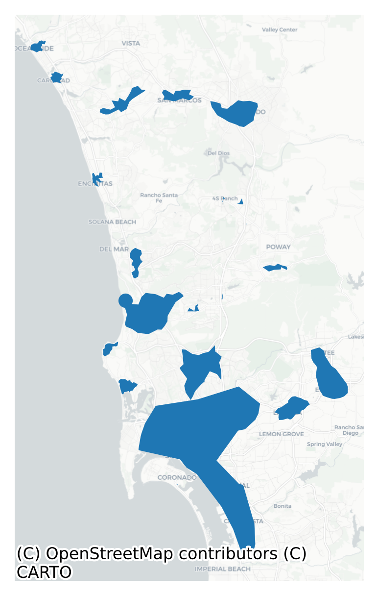
Finally, these are the employment centers we have discovered in the San Diego region using LODES data from 2021. These are groups of intersections in the travel network which belong to a statistically significant spatial cluster of (large) job accessibility. Rather than use census blocks, we’ve represented them using a bespoke polygon that tries to wrap the contained points as tightly as possible.
15.1.3.2 Comparison
For the sake of comparison, we can contrast the employment center polygons identified above against those developed by the San Diego Association of Governments (SANDAG), provided in their open data portal
Employment Centers are identified as areas with a high concentration of employment based on SANDAG’s 2016 employment inventory from Urbansim summarized to quarter-mile radius hexagons. Local-maxima were identified as starting points, and regions were grown to include neighboring hexagons meeting a minimum employment density threshold within an approximate 2-mile radius. The resulting boundaries were generalized (taking into account major barrier features such as topography and freeways) and used to select SANDAG Master Geographic Reference Areas (MGRAs) by activity-weighted (population and employment) centroid. Employment centers are ranked by Tier based on total number of jobs:
Tier 1: 50,000 or more jobs
Tier 2: 25,000 to 49,999 jobs
Tier 3: 15,000 to 24,999 jobs
Tier 4: 2,500 to 14,999 jobs
Hexbin geography (where people live map layers) – generated using a quarter-mile radius hex bin grid overlay on the region. Data is summarized by hex bin spatially using the centroid of an overlying geography.
Where people live by Employment Center they Work In –2015 LEHD census block level data; converted to hexbin (see hexbin geography). LEHD data was used as it contains information on both the home and work location. Data represents an employee residence by the employment center they work in. https://lehd.ces.census.gov/data/.
Make this Notebook Trusted to load map: File -> Trust Notebook
Although the extent of the polygons differ, the accessibility method agrees with the SANDAG employment centers for all centers in Tiers 1-3. With the exception of Carlsbad, Oceanside, and Encinitas, most of SANDAG’s tier 4 centers fail to meet either the density or significant threshold (often both)
In the map below, the access-based employment centers are represented using intersecting census block geometries
Code
m = sandag.explore(tiles="CartoDB Positron")gpd.sjoin(sd_lodes, node_subcenters).dissolve("index_right").explore(color="red", m=m)
Make this Notebook Trusted to load map: File -> Trust Notebook
ignoring the G statistic and looking only at nodes with job access in the top quartile
Code
m = sandag.explore(tiles="CartoDB Positron")lodes_nodes[lodes_nodes.job_rank >0.75].explore(m=m, color="red")
Make this Notebook Trusted to load map: File -> Trust Notebook
When employment accessibility, alone, is the selection criteria (as in the map above), using nodes in the top quintile usually finds the remaining Tier 4 centers, except for some exurban places like Ramona and Otay Mesa
If you really want to be generous, just take the top half of the access distribution
Code
m = sandag.explore(tiles="CartoDB Positron")lodes_nodes[lodes_nodes.job_rank >0.5].explore(m=m, color="red")
Make this Notebook Trusted to load map: File -> Trust Notebook
With this simple rule, we cover all the areas defined by SANDAG, albeit with a much higher resolution
Code
c = center_nodes.groupby('center')['geometry'].apply(lambda x:MultiPoint(x.tolist())).concave_hull(ratio=0.3) gpd.GeoDataFrame(geometry=c, crs=sd_lodes.crs).explore()
Make this Notebook Trusted to load map: File -> Trust Notebook
San Diego Nodes about 50th Job Accessibility Percentile
15.2 Industrial Specialization
Having identified the major employment centers in the San Diego region, a further useful task is characterizing them by their industrial makeup; some centers are likely to be diversified urbanization economies while others are more specialized localization, each of which may leverage different agglomeration forces. Further, center specializations may very by industry, with certain portions of the region specializing in manufacturing with others in finance, and characterizing the centers by these attributes can help planners understand which centers may experience growth or decline given larger macroeconomic patterns.
15.2.1 Concentration Indices
The Herfindahl-Hirschman index (HHI) is a measure of concentration (the inverse of diversity) often used to quantify market share. In ecology, the HHI is used as a kind of segregation measure, where it’s known as Simpson’s Concentration Index, with higher values indicating that a market or area is dominated by a particular producer or species. Here, we are interested in the degree to which the employment in each center is dominated by a single industry.
\[ HHI_c=\sum _{i=1}^{N_{ic}}{ \left( \frac{a_{i_{kc}}}{ \sum{a_{i_{kc}}}}
\right)^{2}}, \] where \(\sum{a_{i_{kc}}}\) is the sum of accessibility values for nodes \(i\) in industry \(k\), located in center \(c\), and \(\sum{a_{i_{kc}}}\) is the sum of accessibility values for all industry categories in nodes located at center \(c\).
Code
# aggregate total employment by center (by NAICS code)center_aggs = ( sd_lodes.drop(columns=["geometry", "geoid", "year"]).groupby("center").sum())# compute Herfindahl indices for each center using NAICS industriesnaics_cols = center_aggs.columns[center_aggs.columns.str.startswith("naics")]hhis = MultiLocalSimpsonConcentration(center_aggs, groups=naics_cols)center_aggs['herf_index'] = hhis.statisticsnode_subcenters_ch.join(pd.Series(hhis.statistics, name='herf_index')).explore("herf_index", tiles="cartodb positron", scheme="user_defined", cmap="RdBu_r", classification_kwds={"bins": [0.01, 0.15, 0.25, 1]}, tooltip=["herf_index"],)
Make this Notebook Trusted to load map: File -> Trust Notebook
From the naked eye, there appears to be a reasonable correlation between HHI and center area; unsurprisingly the centers with the largest footprints are also the most diverse, falling into the first category (blue) classified as urbanization economies. Mid-sized centers are typically classed into the second (orange) bin as mixed economies, with only the very smallest (and only two) centers classified as localization economies.
15.2.2 Location Quotients
The location quotient (LQ) s a measure of industrial specialization in space (Carroll et al., 2008; Isard, 1960; Leigh, 1970). Its simple formula compares the share of employment in a given industry at location \(i\), to the share of that industry’s employment in the region overall. Thus, a LQ greater than one indicates a location has a greater than expected share of an industry, and is relatively specialized.
“For the purposes of detecting industrial specialization, the simple LQ remains the metric of choice.” (Billings & Johnson, 2012)
The location quotient for industry \(k\) in center \(c\) is defined as \[ LQ_{kc} =
\frac{ \left( \frac{\sum^I{a_{i_{kc}}}}{\sum^K\sum^I{a_{i_{kc}}}}\right) }{
\left( \frac{\sum^I{a_{ik}}}{ \sum^K\sum^I{a_{ik}}} \right)}, \] where the numerator \(\left( \sum^I{a_{i_{kc}}} / \sum^K\sum^I{a_{i_{kc}}} \right)\) is the share of accessibility to jobs in industry \(k\) belonging to center \(c\), and the denominator \(\left( \sum^I{a_{i_k}} / \sum^K\sum^I{a_{ik}} \right)\) is the share of access to employment in industry \(k\) for all nodes in the region.
Looking down the columns of the dataframe describes how an industry is concentrated across centers and looking across the rows describes how each center is specialized by industry. To remind ourselves what these categories mean we can use the codebook in the geosnap datastore
Make this Notebook Trusted to load map: File -> Trust Notebook
Billings, S. B., & Johnson, E. B. (2012). The location quotient as an estimator of industrial concentration. Regional Science and Urban Economics, 42(4), 642–647. https://doi.org/10.1016/j.regsciurbeco.2012.03.003
Carroll, M. C., Reid, N., & Smith, B. W. (2008). Location quotients versus spatial autocorrelation in identifying potential cluster regions. The Annals of Regional Science, 42(2), 449–463. https://doi.org/10.1007/s00168-007-0163-1
Cervero, R., & Wu, K.-L. (1998). Sub-centring and Commuting: Evidence from the San Francisco Bay Area, 1980-90. Urban Studies, 35(7), 1059–1076. https://doi.org/10.1080/0042098984484
Duranton, G., & Overman, H. G. (2005). Testing for Localization Using Micro-Geographic Data. The Review of Economic Studies, 72(4), 1077–1106. https://doi.org/10.1111/0034-6527.00362
Enrico, M. (2011). Local Labor Markets. In D. Card & O. Ashenfelter (Eds.), Handbook of Labor Economics (Vol. 4, pp. 1237–1313). Elsevier. https://doi.org/10.1016/S0169-7218(11)02412-9
Getis, A. (1991). Spatial Interaction and Spatial Autocorrelation: A Cross-Product Approach. Environment and Planning A: Economy and Space, 23(9), 1269–1277. https://doi.org/10.1068/a231269
Getis, A., & Ord, J. K. (1996). Local spatial statistics: An overview. Spatial Analysis: Modelling in a GIS Environment, 374.
Giuliano, G., & A. Small, K. (1999). The determinants of growth of employment subcenters. Journal of Transport Geography, 7(3), 189–201. https://doi.org/10.1016/S0966-6923(98)00043-X
Giuliano, G., Redfearn, C., Agarwal, A., & He, S. (2012). Network Accessibility and Employment Centres. Urban Studies, 49(7), 77–95. https://doi.org/10.1177/0042098011411948
Giuliano, G., Redfearn, C., Agarwal, A., Li, C., & Zhuang, D. (2007). Employment concentrations in Los Angeles, 1980-2000. Environment and Planning A, 39(12), 2935–2957. https://doi.org/10.1068/a393
Gordon, P., & Richardson, H. W. (1996). Employment decentralization in US metropolitan areas: Is Los Angeles an outlier or the norm? Environment and Planning A, 28(10), 1727–1743. https://doi.org/10.1068/a281727
Isard, W. (1960). Methods of Regional Analysis: An Introduction to Regional Science. MIT Press.
Knaap, E., Ding, C., Niu, Y., & Mishra, S. (2016). Polycentrism as a sustainable development strategy: Empirical analysis from the state of Maryland. Journal of Urbanism: International Research on Placemaking and Urban Sustainability, 9(1), 73–92. https://doi.org/10.1080/17549175.2015.1029509
Knaap, E., & Rey, S. (2024). Measuring two decades of urban spatial structure: The evolution of agglomeration economies in American metros. Computers, Environment and Urban Systems, 110, 102116. https://doi.org/10.1016/j.compenvurbsys.2024.102116
Leigh, R. (1970). The Use of Location Quotients in Urban Economic Base Studies. Land Economics, 46(2), 202. https://doi.org/10.2307/3145181
McDonald, J. F., & McMillen, D. P. (2000). Employment Subcenters and Subsequent Real Estate Development in Suburban Chicago. Journal of Urban Economics, 48(1), 135–157. https://doi.org/10.1006/juec.1999.2160
Ord, J. K., & Getis, A. (1995). Local Spatial Autocorrelation Statistics: Distributional Issues and an Application. Geographical Analysis, 27(4), 286–306. https://doi.org/10.1111/j.1538-4632.1995.tb00912.x
Proost, S., & Thisse, J.-F. (2019). What Can Be Learned from Spatial Economics? Journal of Economic Literature, 57(3), 575–643. https://doi.org/10.1257/jel.20181414