Segregation is in many ways the core of urban inequality research; any discussion of urban analytics is incomplete without decent coverage of segregation measurement. One of the most obvious and long-studied avenues for creating inequality between groups is to partition access to different resources. This is also one of the most important legacies of institutionalized racism in the United States, where the unequal distribution of public resources has repeatedly been shown to be illegal. In other words, there is an important legacy of urban inequality research closely related to legal challenges against federal policy; if policies governing public resources (like education, housing, transportation infrastructure, clean air and water, etc.) result in segregation (for some protected class), then they are inherently unequal (and ultimately unconstitutional, thanks to the equal protection clause).
Segregation of white and colored children in public schools has a detrimental effect upon the colored children. The impact is greater when it has the sanction of the law, for the policy of separating the races is usually interpreted as denoting the inferiority of the Negro group… Any language in contrary to this finding is rejected. We conclude that in the field of public education the doctrine of ‘separate but equal’ has no place. Separate educational facilities are inherently unequal.
In concept, segregation is about separation; when we measure residential segregation, we are asking whether people belonging to different groups share the same space, often conceived as the same ‘neighborhood’. This is a more ambiguous task than measuring, for example, educational segregation, where the shared resource such as schools are very well-defined. Residential space can be measured at the scale of the room, housing unit, building, collection of buildings, neighborhood, city, region, and all the way on (we explore this variable concept of scale in the next section).
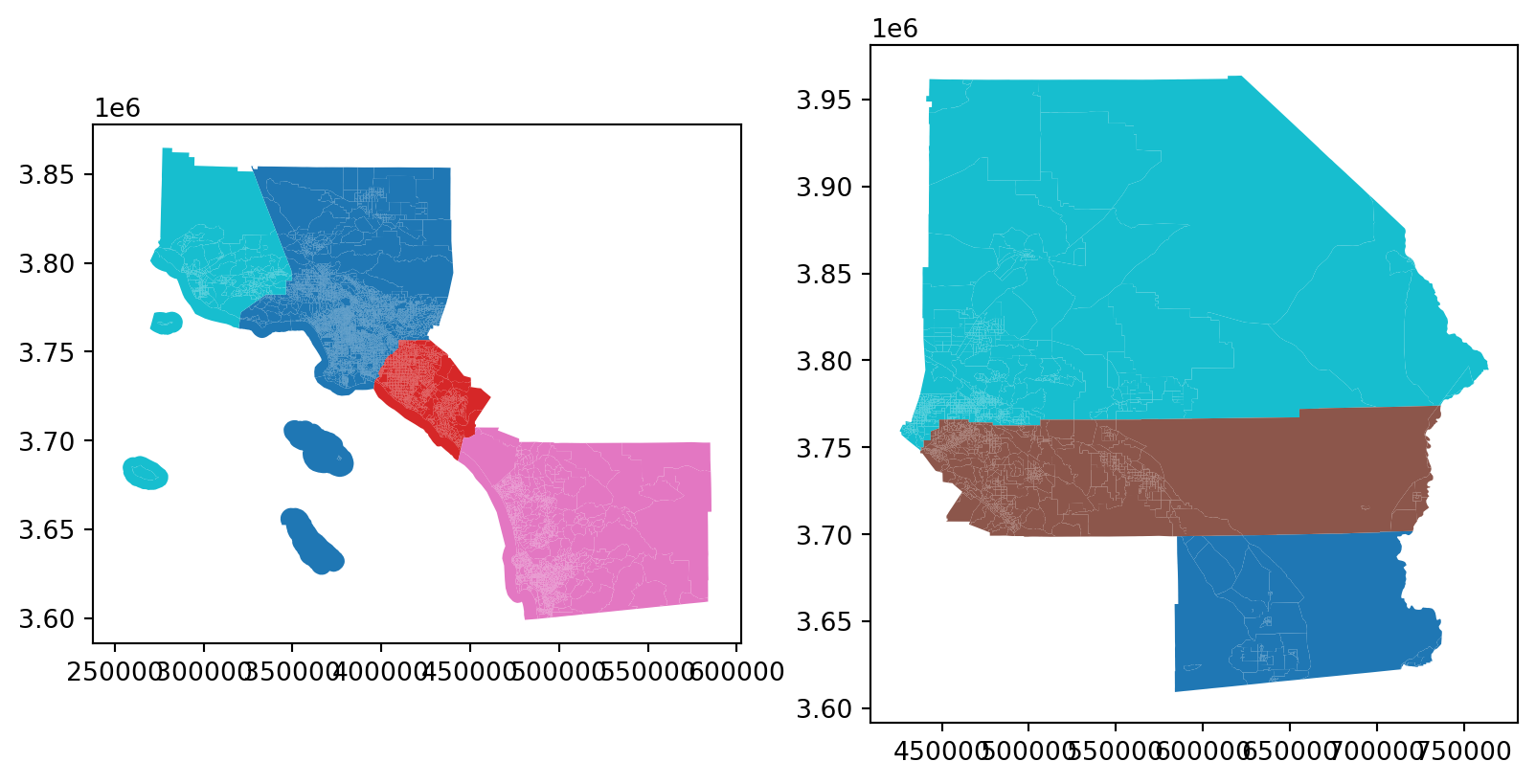
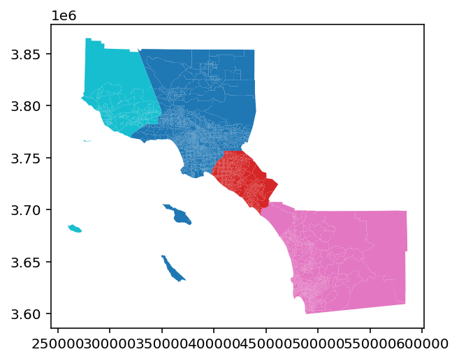
Thus in the case of residential segregation we are forced to rely on the fuzzy notion of neighborhoods. In practice, this means that researchers simply adopt the tract or blockgroup as a placeholder for the neighborhood, then examine segregation as defined by these units. Here, we’ll use PySAL’s segregation module to analyze residential segregation by race and ethnicity in Southern California, and we begin by collecting data for the entire region, then partitioning it into the coastal and inland sections.
/Users/knaaptime/miniforge3/envs/urban_analysis/lib/python3.12/site-packages/geosnap/io/constructors.py:218: UserWarning: Currency columns unavailable at this resolution; not adjusting for inflation
warn(
Coastal and Inland Southern California
16.1 Residential Segregation Measures
The segregation package calculates dozens of segregation indices, each of which captures something different about the ways that population groups interact or remain separated in space. Most of the commonly-used statistics are global or aggregate measures, meaning they summarize the total level of segregation across all units in a study region. For an overview of segregation measure nomenclature, formulae, and canonical citations, see the tables at the end of Grannis (2002).
16.1.1 Single-Group Indices
Single-group indices measure the partitioning of one population group relative to everyone else. Early segregation work in the U.S. tends to focus on Black-white segregation, but it is also common to see work focused on a particular minority population versus the rest of the population (e.g. Black vs all other groups). To generate a single-group measure using the segregation package, you pass a dataframe holding population counts for each geographic unit, and the names of the columns for the focal population and the reference population (i.e. the minority the total population).
Here, we fit three segregation measures: Dissimilarity (\(D\)), Gini (\(G\)), and Entropy (also called the Information Theory index, sometimes denoted [Thiel’s] \(H\)) for the Black population and the Hispanic/Latino populations in the southern California region. Each class has a statistic attribute that holds the computed value for each segregation measure.
Code
dissim_hisp.statistic
np.float64(0.4995777695234679)
Code
dissim_black.statistic
np.float64(0.547197680270968)
Code
gini_hisp.statistic
0.6602166788700566
Code
gini_black.statistic
0.7234615852802052
Code
entropy_hisp.statistic
np.float64(0.2714618709533524)
Code
entropy_black.statistic
np.float64(0.2616509031724341)
According to the Dissimilarity and Gini indices, the black population in southern California is more segregated than the Latinx/Hispanic population, but the reverse is true according to the Entropy index.
16.1.1.1 Batch Computation
To examine several indices at once, segregation provides a set of “batch_compute” functions. Instead of a fitted Class, the batch_compute_singlegroup function returns a table of segregation indices and is a convenient way of collecting many statistics simultaneously.
Multi-group measures capture the partitioning of several population groups simultaneously. Most multi-group measures are extensions of single-group measures and have a more recent history in the literature (Reardon & Firebaugh, 2002).
Regardless which index is used, multigroup segregation is higher in the coastal region than the inland one
16.1.2.1 Batch Computation
Again, the measures can be “batch computed”
Code
socal_all_multigroup
Statistic
Name
GlobalDistortion
335.5186
MultiDissim
0.5131
MultiDivergence
0.3498
MultiDiversity
1.1664
MultiGini
0.6766
MultiInfoTheory
0.2999
MultiNormExposure
0.3048
MultiRelativeDiversity
0.2955
MultiSquaredCoefVar
0.2508
SimpsonsConcentration
0.3517
SimpsonsInteraction
0.6483
16.1.3 Local Segregation Measures
Unlike global measures, local segregation statistics measure segregation in each geographic unit rather than summarizing segregation across the region. For example the recently proposed Distortion index is designed to visualize how segregation changes over a region (Bézenac et al., 2022; Olteanu et al., 2019).
The use of trajectory convergence analysis provides a flexible way for capturing change across all scales from small spatial units and how the rate of convergence to the citywide average modifies over space. Thus, the method provides an analysis of how far, in spatial terms, any individual or neighborhood is from the citywide multigroup distribution.
Make this Notebook Trusted to load map: File -> Trust Notebook
16.2 The Dimensions of Residential Segregation
With more than 20 segregation indices at our disposal, it can be confusing to understand which measure is ‘best’ or whether multiple indices really capture slightly different versions of ‘the same thing’. A seminal contribution in segregation measurement is given by Massey & Denton (1988) who were the first to examine quantitatively the wide variety of segregation indexing strategies and the information each provides. Their paper is important first because of the sheer volume of work: in the late 80s, it was seriously laborious to gather data for a large number of metropolitan regions and compute a dozen segregation indices in each one; the paper’s second major contribution is the way it helped clarify the relationships among various indices that had been proposed over the years.
Like personality theory and item-response theory in psychology, Massey and Denton proposed that there were multiple ways to measure segregation that capture different concepts of the term (i.e. unevenness versus clustering)–but there probably are not 20 different concepts like there are indices in use. Instead, those two dozen indices are different ways of capturing the five or so dimensions of segregation that really exist (they argue). This was a dramatic step forward in understanding what we’re actually measuring when we study residential segregation. To conduct their analysis, Massey and colleagues gathered metropolitan data from around the country and computed every segregation index they could manage, then they ran a factor analysis on the set of results.
Assessing the outcome, they argued that segregation indices could be divided into five categories: evenness, exposure, concentration, centralization, and clustering.
Minority members may be distributed so that they are overrepresented in some areas and underrepresented in others, varying on the characteristic of evenness. They may be distributed so that their exposure to majority members is limited by virtue of rarely sharing a neighborhood with them. They may be spatially concentrated within a very small area, occupying less physical space than majority members. They may be spatially centralized, congregating around the urban core, and occupying a more central location than the majority. Finally, areas of minority settlement may be tightly clustered to form one large contiguous enclave, or be scattered widely around the urban area. (Massey & Denton, 1988, p. 283)
Following Massey & Denton (1988), Massey et al. (1996), and Massey (2012) we can look at dimensionality in segregation measures by computing two-group indices for Black, Hispanic, and Asian groups (vs all others) for every metro region in the country. Here we will use the 2021 ACS data at the blockgroup level, and use a 2km radius for computing generalized spatial measures, which helps account for heterogeneity in BG size
Code
multi_groups = ["n_nonhisp_white_persons","n_nonhisp_black_persons","n_hispanic_persons","n_asian_persons",]singles = ["n_nonhisp_black_persons", "n_hispanic_persons", "n_asian_persons"]datasets = DataStore()msas = datasets.msas()msas = msas[msas["type"].str.startswith("Metro")] # only metros not microsmsa_fips = msas.geoid.values
16.2.1 Two-Group Measures
To recreate Massey’s results, we will batch compute every segregation index available in a for-loop using data for every metropolitan region in the country. This gives us the raw data we need to ask whether the indices can be collapsed into a smaller set of factors.
Code
for group in singles:ifnot os.path.exists(f"../data/{group}_measures.csv"): dfs = []for metro in msa_fips:try:# get blockgroup-level data for the MSA df = gio.get_acs(datasets, msa_fips=metro, level="bg", years=[2021])# create a temporary 'total' population of white/other df["temp_total"] = df[group] + df["n_nonhisp_white_persons"] df = df.dropna(subset=["geometry"]).to_crs(df.estimate_utm_crs())# compute all seg measures with a 2km neighborhood seg = batch_compute_singlegroup( df, group_pop_var=group, total_pop_var="temp_total", distance=2000 ) dfs.append(seg.Statistic.rename(metro))exceptExceptionas e: # PR will failprint(e) df =Nonepass results = pd.concat(dfs, axis=1).T results.to_csv(f"../data/{group}_measures.csv")results = pd.concat( [pd.read_csv(f"../data/{group}_measures.csv", index_col=0, converters={0:str}) for group in singles])
The results dataframe now stores every segregation index for every metropolitan region in the country, with each row representing a different metro region and each column storing a different segregation index. As such, we could use it to quickly glance at the most segregated places in the country in 2021. According to the Gini index, the top ten were essentially all in the South or the Midwest.
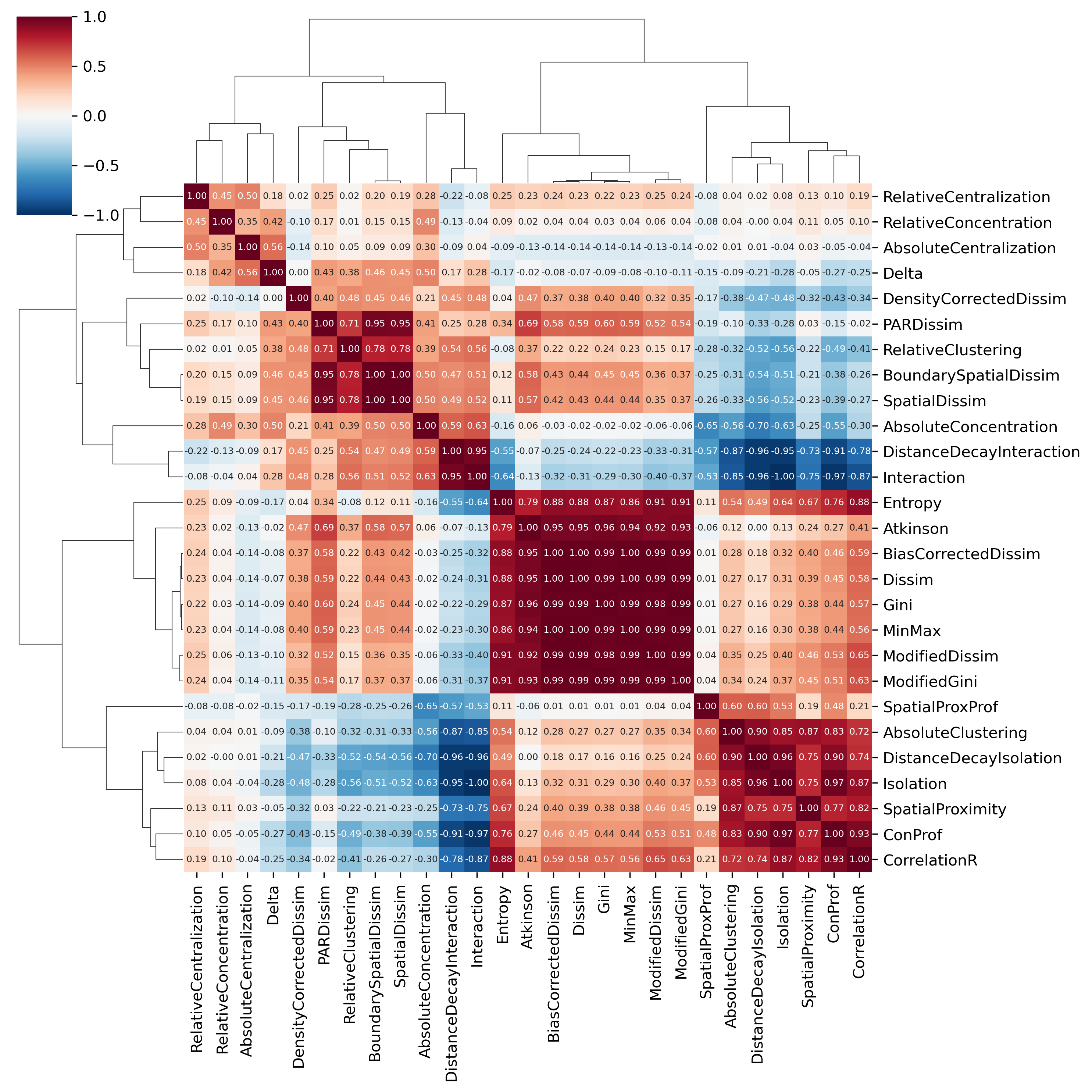
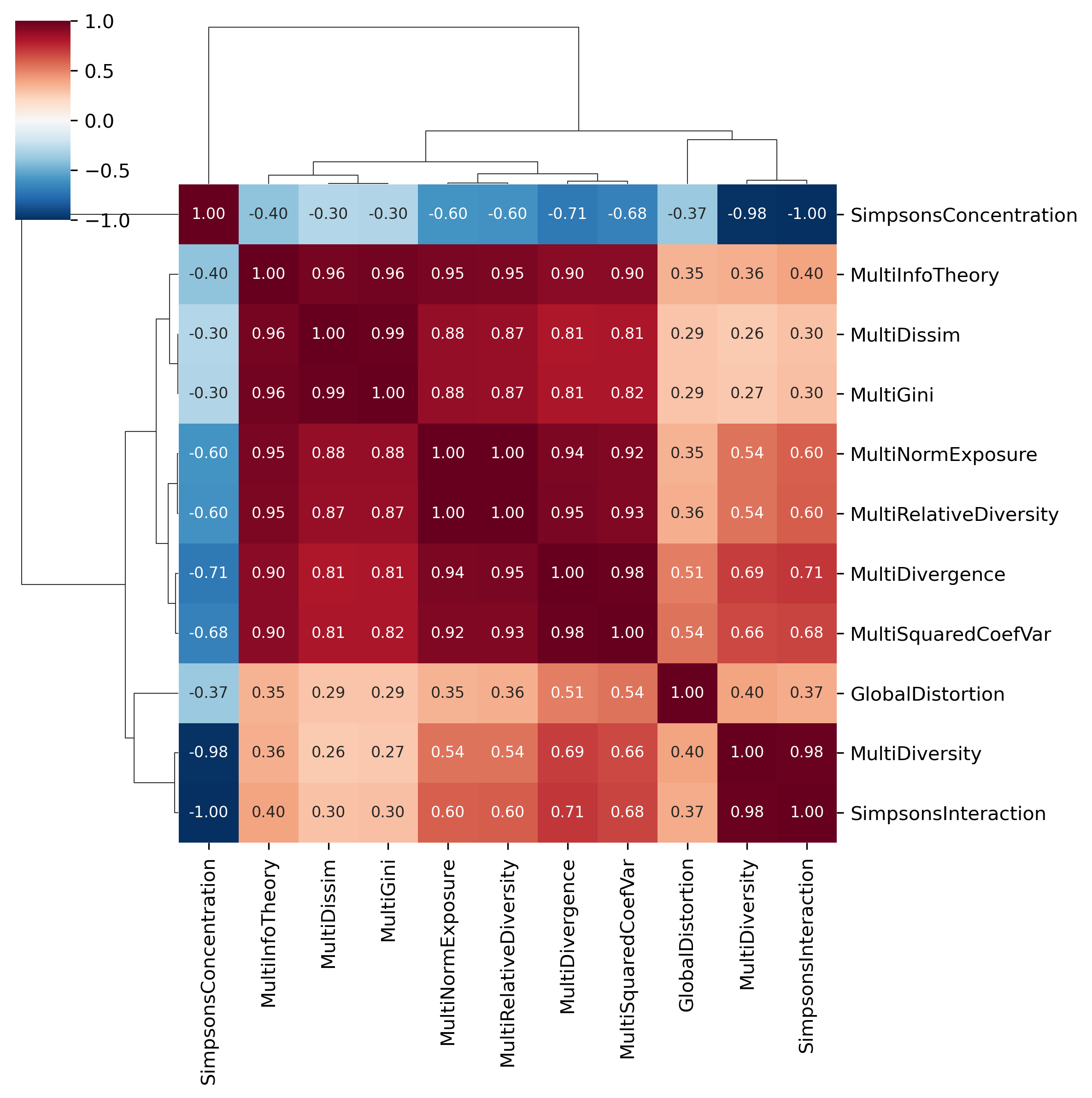
One of the easiest ways to understand the dimensionality in the dataset is a heatmap of the variable correlation matrix, which we can do using the clustermap function from seaborn. A good way to pick out groups of variables is to scan the diagonal for blocks of red.
The large contiguous blocks are groups of variables that are highly intercorrelated, and capture largely the “same thing”. Whether the underlying concept being measured is a factor or a component is a matter of debate. In the segregation context, these different indices are probably better treated as components that capture slightly different measurements of the same construct, rather than manifest outcomes of some underlying latent process of, e.g. “unevenness segregation”. That is, the Gini and Dissimilarity indices are probably different ways of measuring ‘unevenness’, as opposed to a social process of unevenness that manifests as these two different variables, “gini” and “dissimilarity”… As Rees (1971) describes, factor analysis applied to urban data more often adopts the alternative: “more modest is the claim that components or factors represent concise descriptions of patterns of associations of attributes across observations.”
All the same, the Massey and Denton approach that treats dimensions as factors is a useful way of tackling the problem, and we can adopt the factor view to recreate their analysis.
Factor analysis is an attempt to approximate a correlation or covariance matrix with one of lesser rank. The basic model is that \(_nR_n \approx _n F_{kk}F'_n + U^2\) where \(k\) is much less than \(n\). There are many ways to do factor analysis, and maximum likelihood procedures are probably the most commonly preferred (see factanal )… If variables are thought to represent a “true” or latent part then factor analysis provides an estimate of the correlations with the latent factor(s) representing the data. If variables are thought to be measured without error, then principal components provides the most parsimonious description of the data.
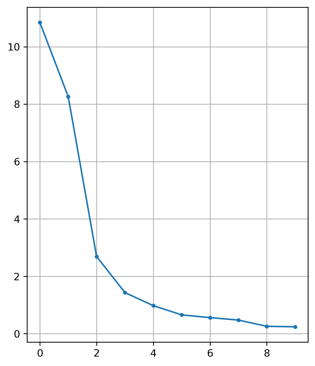
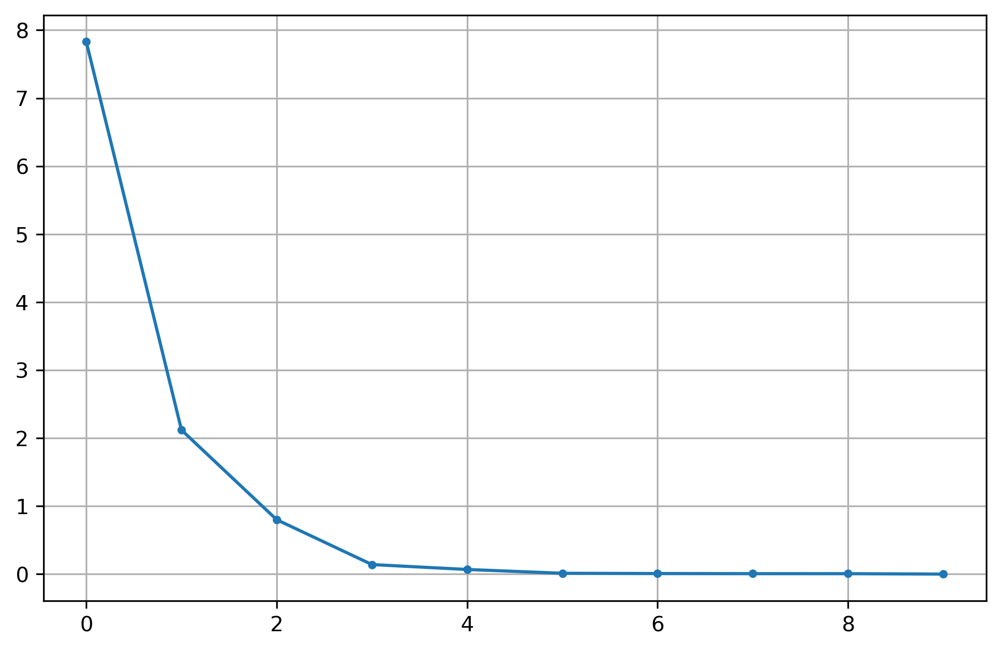
To assess the number of factors we need to extract, it is common to begin exploratory factor analyses with a ‘scree plot’. Here, we fit the same number of factors as variables in the data, then plot the amount of variance accounted by each factor. Moving to the right along the x-axis, we are looking for an “elbow” in the plot that shows where estimating additional factors does not explain much more variance.
Code
# first look for n_factors)fa = FactorAnalyzer(rotation="oblimin", n_factors=results.shape[1])fa.fit(results.fillna(0))ev, v = fa.get_eigenvalues()ev = pd.Series(ev)ev.iloc[:10].plot(grid=True, style=".-", figsize=(5,6))
/Users/knaaptime/miniforge3/envs/urban_analysis/lib/python3.12/site-packages/sklearn/utils/deprecation.py:132: FutureWarning: 'force_all_finite' was renamed to 'ensure_all_finite' in 1.6 and will be removed in 1.8.
warnings.warn(
Scree-Plot of Segregation Factors
The scree plot suggests an albow at about 3, maybe 4. Revelle says do not use the eigenvalue >1 rule to determine n_factors
/Users/knaaptime/miniforge3/envs/urban_analysis/lib/python3.12/site-packages/sklearn/utils/deprecation.py:132: FutureWarning: 'force_all_finite' was renamed to 'ensure_all_finite' in 1.6 and will be removed in 1.8.
warnings.warn(
loadings less than .1 are considered unimportant (R and others suppress them). Revelle says ignore less than .3.
We will follow Massey and Denton and the clustering results above, and shoot for 5 factors
Code
factors = factors.mask(factors <0.3)factors
F1
F2
F3
F4
F5
AbsoluteCentralization
NaN
NaN
NaN
NaN
0.717832
AbsoluteClustering
NaN
NaN
0.695828
0.475336
NaN
AbsoluteConcentration
NaN
NaN
NaN
NaN
0.314571
Atkinson
0.927950
NaN
NaN
NaN
NaN
BiasCorrectedDissim
0.975286
NaN
NaN
NaN
NaN
BoundarySpatialDissim
NaN
0.866075
NaN
NaN
NaN
ConProf
0.329183
NaN
0.560560
NaN
NaN
CorrelationR
0.481336
NaN
0.670719
NaN
NaN
Delta
NaN
0.626410
NaN
NaN
0.424750
DensityCorrectedDissim
0.526844
NaN
NaN
NaN
NaN
Dissim
0.974563
NaN
NaN
NaN
NaN
DistanceDecayInteraction
NaN
NaN
NaN
NaN
NaN
DistanceDecayIsolation
NaN
NaN
0.526268
0.528260
NaN
Entropy
0.815438
NaN
0.377583
NaN
NaN
Gini
0.971297
NaN
NaN
NaN
NaN
Interaction
NaN
NaN
NaN
NaN
NaN
Isolation
NaN
NaN
0.516079
0.360120
NaN
MinMax
0.974450
NaN
NaN
NaN
NaN
ModifiedDissim
0.968980
NaN
NaN
NaN
NaN
ModifiedGini
0.972560
NaN
NaN
NaN
NaN
PARDissim
0.311544
0.859431
NaN
NaN
NaN
RelativeCentralization
0.314008
NaN
NaN
NaN
0.725198
RelativeClustering
NaN
0.780695
NaN
NaN
NaN
RelativeConcentration
NaN
NaN
NaN
NaN
0.588542
SpatialDissim
NaN
0.857307
NaN
NaN
NaN
SpatialProxProf
NaN
NaN
NaN
0.864273
NaN
SpatialProximity
NaN
NaN
0.876189
NaN
NaN
The latent factors are on the columns and the loadings for each variable are on the rows
Code
for f in factors.columns:print(f"{f}:\n",factors.dropna(subset=[f])[f].sort_values(ascending=False),"\n")
The phi_ attribute stores the factor correlation matrix, which looks pretty reasonable here. There is some correlation among the factors (as expected, since we used an oblique transform, intentionally), but nothing that looks overlapping. In other words, while the factors look like they may be related, each one is capturing unique information as well
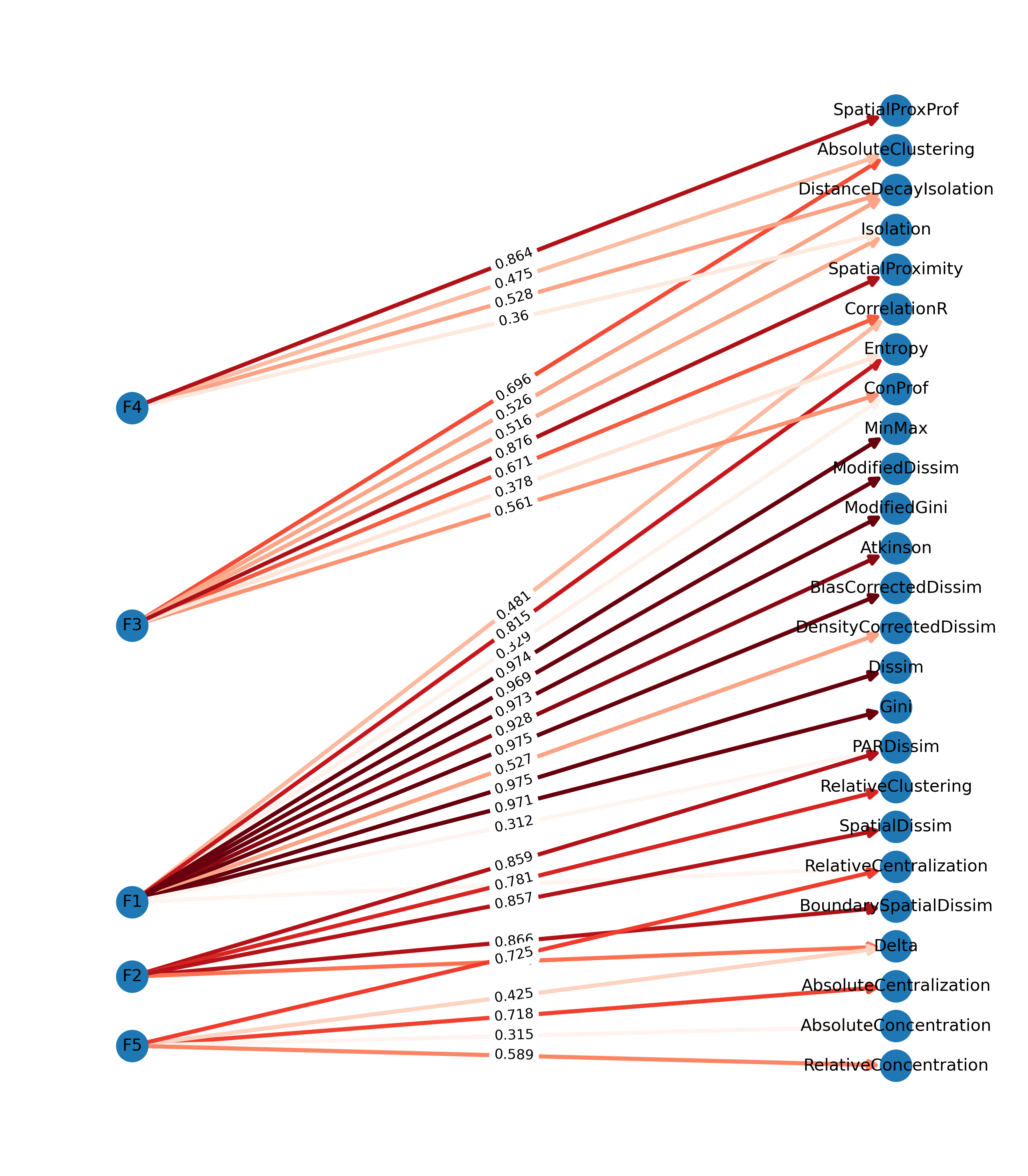
A common visualization technique for factor analysis is to create path diagrams which show the relationship between input variables and the latent factors. The factor analysis ecosystem is a lot less developed in Python than it is in R, but we can recreate a typical visualization using networkx and pygraphviz, (specifically, by slightly tweaking the dot layout). First, we convert the factor loadings to a networkX network object, where the factors and variables are nodes in a hierarchical directed network, and the factor loadings represent the edge weights between factors and variables, then we use the graphviz dot layout to draw the graph
Code
G2 = nx.from_pandas_edgelist( factors.T.stack().rename("weight").reset_index().round(3), source="level_0", target="level_1", edge_attr="weight", edge_key="weight", create_using=nx.DiGraph,)f, ax = plt.subplots(figsize=(13, 15))pos = graphviz_layout(G2, prog="dot", args='-Grankdir="LR"')nx.draw_networkx( G2, pos=pos, with_labels=True, ax=ax, edge_cmap=plt.cm.Reds, edge_color=factors.T.stack().values, node_size=500, width=3, arrowsize=14,)labels = nx.get_edge_attributes(G2, "weight")nx.draw_networkx_edge_labels(G2, pos, edge_labels=labels)ax.margins(0.1, None) # add some horizontal space to fit labelsax.axis('off')plt.show()
Segregation Measure Factor Loading Graph
This plot shows the relationship between factors and variables as a kind of network graph. In this case, each of the factors is displayed as a node on the lefthand side and arrows point to each of the variables that load strongly onto the factor (with color and label denoting intensity). The direction of the arrow is important as it implies that the measured variables are partial outcomes from the latent factor.
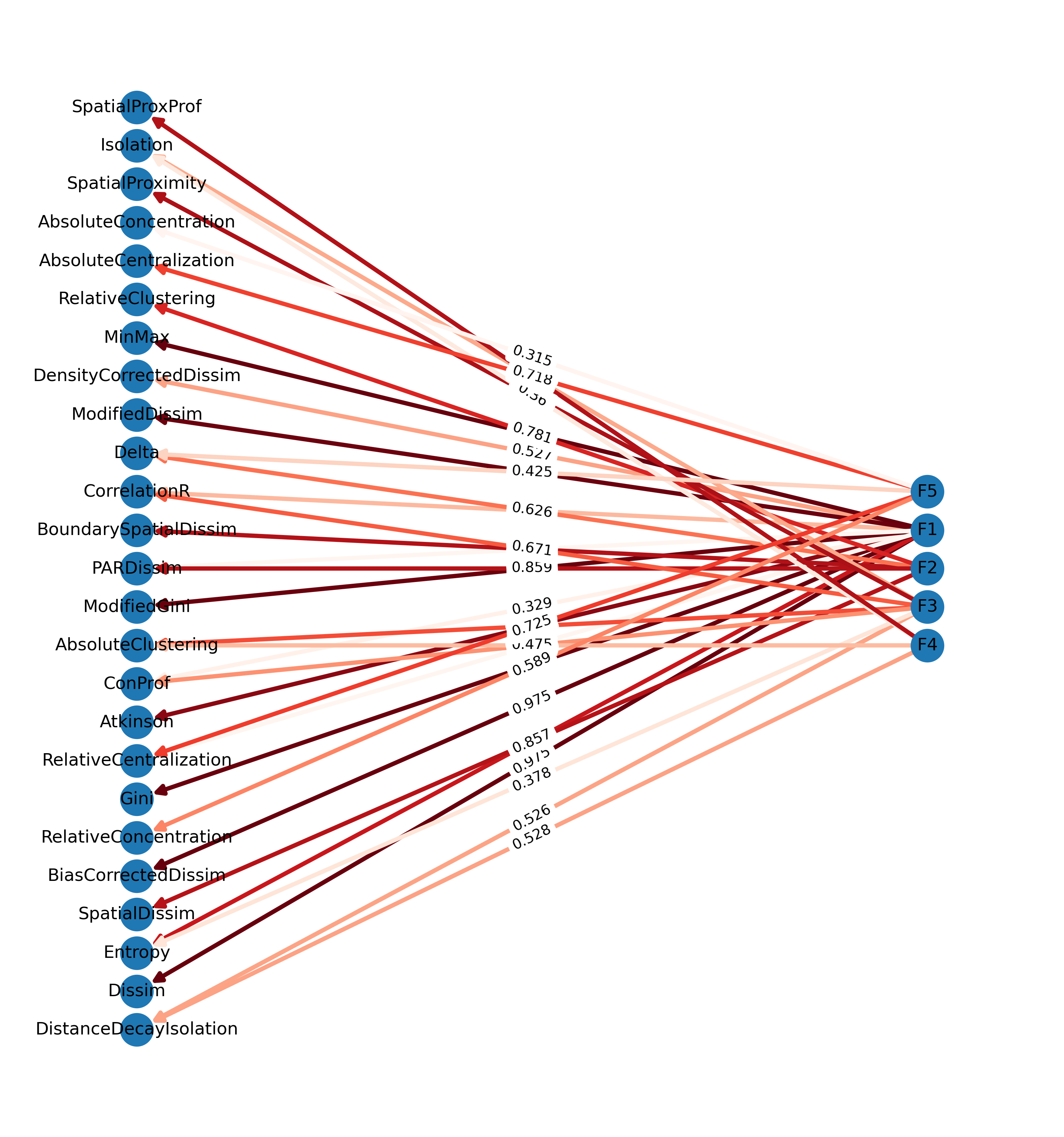
This graphic can also be done in pure networkx (i.e. without pygraphviz) using a multipartite layout, but the result is not as nice because it doesnt group the manifest variables to avoid line crossings, and the latent variables all have the same spacing, which increases overlap
Code
f, ax = plt.subplots(figsize=(13, 14))for layer, nodes inenumerate(reversed(tuple(nx.topological_generations(G2)))):# `multipartite_layout` expects the layer as a node attribute, so add the# numeric layer value as a node attributefor node in nodes: G2.nodes[node]["layer"] = layer# Compute the multipartite_layout using the "layer" node attributepos = nx.multipartite_layout( G2, subset_key="layer", align="vertical",)nx.draw_networkx( G2, pos=pos, ax=ax, edge_cmap=plt.cm.Reds, edge_color=factors.T.stack().values, node_size=500, width=3, arrowsize=14,)nx.draw_networkx_edge_labels(G2, pos, edge_labels=labels)ax.margins(0.1, None) # add some horizontal space to fit labelsax.axis('off')
Instead of factor analysis, we could alternatively use cluster analysis to try and group segregation indices into categories.
Affinity propagation is a clustering algorithm where k is endogenous so it works well for exploratory analysis when we are not sure about the number of clusters. If we fit a cluster model to the correlation matrix of segregation indices, we’re looking for groups of variables that capture the same dimension. This works for our purposes here because we don’t really care about the factor loadings or measuring the latent construct per se (the segregation measures themselves are preferable for that). Instead, we’re asking whether these indices are providing unique information, and how many unique dimensions should we consider?
Since cluster assignments are discrete, and we think of cluster assignments as ‘best’ when they are unambiguous (i.e. clusters are well-separated and each observation belongs to only one cluster), this is like treating the dimensions as orthogonal in factor analysis… If we think the factors are correlated (oblique rotated), then the clusters wouldn’t be well-separated.
Code
ap = AffinityPropagation().fit_predict(results.corr())ap = pd.Series(dict(zip(results.columns.values, ap)), name="Index Type")ap.nunique()
The interesting thing is how well these results map onto Massey and Denton’s originals, despite the idea that clustering and exposure make more sense collapsed into a single category (that concept seems even more pronounced in these results, since isolation and interaction are basically inverses, but end up in different categories)
The clustering algorithms are all really stable in their assignments. When you tune hierarchical and kmeans using the optimal silhouette score, they agree on the exact assignments in the 5 cluster solution
16.2.4 Multi-Group Measures
Following, we can extend Massey et al’s analysis to multigroup segregation indices
Code
ifnot os.path.exists(f"../data/multigroup_measures.csv"): dfs = []for metro in msa_fips:try: df = gio.get_acs(datasets, msa_fips=metro, level="bg", years=[2021]) df = df.dropna(subset=["geometry"]).to_crs(df.estimate_utm_crs()) seg = batch_compute_multigroup(df, groups=multi_groups, distance=2000) dfs.append(seg.Statistic.rename(metro))exceptExceptionas e: # PR will failprint(e) df =Nonepass results = pd.concat(dfs, axis=1).T results.to_csv(f"../data/multigroup_measures.csv")
Heatmap of Multigroup Segregation Measure Correlation Matrix
Code
famulti = FactorAnalyzer(rotation="oblimin", n_factors=results_multi.shape[1])famulti.fit(results_multi.fillna(0))ev, v = famulti.get_eigenvalues()ev = pd.Series(ev)ev.iloc[:10].plot(grid=True, style=".-")
/Users/knaaptime/miniforge3/envs/urban_analysis/lib/python3.12/site-packages/sklearn/utils/deprecation.py:132: FutureWarning: 'force_all_finite' was renamed to 'ensure_all_finite' in 1.6 and will be removed in 1.8.
warnings.warn(
In practice, we have seen that segregation can compute two dozen segregation indices, but many of them capture the same concept. This yields a simple question, which index is most appropriate for studying e.g. racial and ethnic segregation in the city? There is no single answer for that question, but the literature has good suggestions about the best defaults. In particular, Reardon & Firebaugh (2002) examine the mathematical properties of many multigroup measures, arguing that the information theory index (\(H\)) and isolation index (what they term \(P\ast\)) have the most attractive features for capturing evenness and exposure/isolation, respectively.
the spatial exposure/isolation index \(\tilde{P\ast}\) which can be interpreted as a measure of the average composition of individuals’ local spatial environments–and the spatial information theory index \(\tilde{H}\) which can be interpreted as a measure of the variation in the diversity of the local spatial environments of each individual—are the most conceptually and mathematically satisfactory of the proposed spatial indices.
In the segregation package, the singlegroup and multigroup classes for these measures are Entropy and MultiInfoTheory for \(H\), and Isolation/Exposure and MultiNormExposure for \(P\ast\). In the next section we examine spatial segregation indices which provide more explicit avenues for assessing centralization, concentration, and clustering, as well as methods that incorporate space into the entropy and isolation measures in flexible and realistic ways.
Bézenac, C., Clark, W. A. V., Olteanu, M., & Randon‐Furling, J. (2022). Measuring and Visualizing Patterns of Ethnic Concentration: The Role of Distortion Coefficients. Geographical Analysis, 54(1), 173–196. https://doi.org/10.1111/gean.12271
Grannis, R. (2002). Discussion: Segregation Indices and Their Functional Inputs. Sociological Methodology, 32(1), 69–84. https://doi.org/10.1111/1467-9531.00111
Massey, D. S., & Denton, N. A. (1988). The Dimensions of Residential Segregation. Social Forces, 67(2), 281–315. https://doi.org/10.1093/sf/67.2.281
Massey, D. S., White, M. J., & Phua, V.-C. (1996). The Dimensions of Segregation Revisited. Sociological Methods & Research, 25(2), 172–206. https://doi.org/10.1177/0049124196025002002
Olteanu, M., Randon-Furling, J., & Clark, W. A. V. (2019). Segregation through the multiscalar lens. Proceedings of the National Academy of Sciences, 116(25), 12250–12254. https://doi.org/10.1073/pnas.1900192116
Rees, P. H. (1971). Factorial Ecology: An Extended Definition, Survey, and Critique of the Field. Economic Geography, 47(4), 220. https://doi.org/10.2307/143205
Revelle, W. (2024). Psych: Procedures for psychological, psychometric, and personality research [Manual]. Northwestern University. https://CRAN.R-project.org/package=psych