Code
import collections.abc
# hacky but necessary until a new pylogit is out
= collections.abc.Iterable
collections.Iterable
import choicemodels
import geopandas
import pandas
import pylogit
import collections.abc
# hacky but necessary until a new pylogit is out
= collections.abc.Iterable
collections.Iterable
import choicemodels
import geopandas
import pandas
import pylogit
If you want to be good at urban choice modeling, go study with civil engineers and transportation modelers. See McFadden & Reid (1975), McFadden (1978), Anas (1980), Anas (1981), Anas (1983), Anas (1984), Anas (1985), Ben-Akiva & Bierlaire (1999), McFadden & Train (2000), Donnelly et al. (2010), Koppelman & Bhat (2006), Páez & Boisjoly (2022), Bhat & Guo (2004), Bhat & Koppelman (2006), Bhat (1997), Bhat & Guo (2007), Guo & Bhat (2007), Pinjari et al. (2007), Rajamani et al. (2003), Jeffrey Newman’s transportation modeling course, or Michael Clark’s Categorical Regression Models course. The classic (and open) textbook is Train (2001), and Hensher et al. (2015) is a great, accessible, modern textbook.
Transportation modeling is a huge field, partly because it is well-funded by the federal government. Although integrated land-use/transportation models are part of the DNA of urban studies and regional science, land-use models (especially residential location-choice models) have received less attention (which is not to say the field is underdeveloped) (Batty, 1972; Benenson, 2004; Harris, 1985, 1994; Harris & Batty, 1993; Kain, 1987; Pagliara et al., 2010; Pinjari et al., 2007). Location-choice models of land-use take a different form than the CA models of land-use we explored in Chapter 30 because we try to explicitly model demand from a behavioral perspective, rather than treat observations as automata.
“Simulation models of residential location meet several of our criteria for good models, failing partially on the question of behavioral realism, and most seriously with respect to social and ethnic externalities. Their theoretical and economic content is well-conceived, and they have begun to accommodate discrete choice behavior. The marriage between social science theory and simulation is not yet as secure as might be desired, and on many fronts much work remains to be done.
– Harris (1985)
A residential location choice model is similar to a destination choice model in transportation research because there are dozens–maybe thousands of options in the choice set (unlike, say, a mode-choice model where there are only a handful of alternatives)
The crucial difference between location choice models and for example mode or destination choice models is that each of the alternatives is actually chosen by some household (in equilibrium). This is a significant difference from, say, mode choice models, where we are able to include alternatives chosen by nobody by generating them from travel supply data. In fact, were it not for differences across households such as income and family characteristics, the observable part of the utility ui would be the same for all residences, assuming market equilibrium prices. Generalized travel costs and environmental characteristics will be capitalized into housing prices. Thus, it is evident that the explaining power of the model is largely determined by how finely described the households are, as opposed to, say, mode choice models, where the travel time and travel cost of an alternative is often able to explain the observed choices to a large extent.
– Eliasson (2010)
Brathwaite & Walker (2018)
Notwithstanding the name, we generally view the parameters of a location ‘choice’ model as sorting influences rather than strict preferences (Quillian, 2015)
One important lesson from the last half-century of large-scale modeling exercises in the U.S. is that you cannot use models based on AI and ML to conduct scenario analysis for practical planning purposes (Lee, 1973; Spiekermann & Wegener, 2018). This modeling framework (e.g. the kind setup in Chapter 30) is interesting for exploration but impractical for policy development because (1) they are inaccurate and (2) the public distrusts them. In the first place, these models are not built on behavioral assumptions, so they do not accurately predict behavior in the future when scenario inputs are changed and simulated forward. In most cases, you need a structural modeling approach that assumes agents behave according to some behavioral principle (like utility maximization)–which is why McFadden (1978) won the Nobel prize (Manski, 2001). The discrete choice model famously provided far superior out-of-sample predictions for BART ridership than the prior generation of predictive models because it turns out to be a pretty accurate structural model of social behavior that is well-suited for policy analysis (Heckman & Vytlacil, 2007a; Heckman & Vytlacil, 2007b; Koopmans, 1949; Pearl, 1998)
Following, the best urban models rely on structural estimation (Holmes & Sieg, 2015) and require very thorough subject knowledge; this is essentially the antithesis of AI1. Second, urban planners have long rejected governance via computer overlord. Thus the point of modern scenario planning exercises is not only to develop simulated predictions under different growth assumptions, but also to communicate those findings to a constituency of residents and policymakers (Hopkins, 2014; Hopkins, 1974; Hopkins & Knaap, 2019; Hopkins & Zapata, 2007; Kaza & Hopkins, 2012; Klosterman, 1994; Knaap et al., 2020; Knaap et al., 1998; Spiekermann & Wegener, 2018). Good luck explaining that Deep Net (and soliciting buy-in) at your next planning commission meeting.
Metropolitan Planning Agencies needed models to assess the consequences of alternative transportation plans and policies on urban development and travel patterns. Some wanted to evaluate the effects of land policies such as the use of urban growth boundaries, or policies to promote transit-oriented development. Most wanted to be able to address these kinds of policy analysis questions with models that were behaviorally clear and as transparent as possible, avoiding the problems identified three decades ago by Lee’s critical assessment of the state of large scale urban simulation (Lee 1973), and the more general skepticism of “black-box” models that were so complex that their logic could not be explained to policy-makers or the public.
– Waddell (2010)
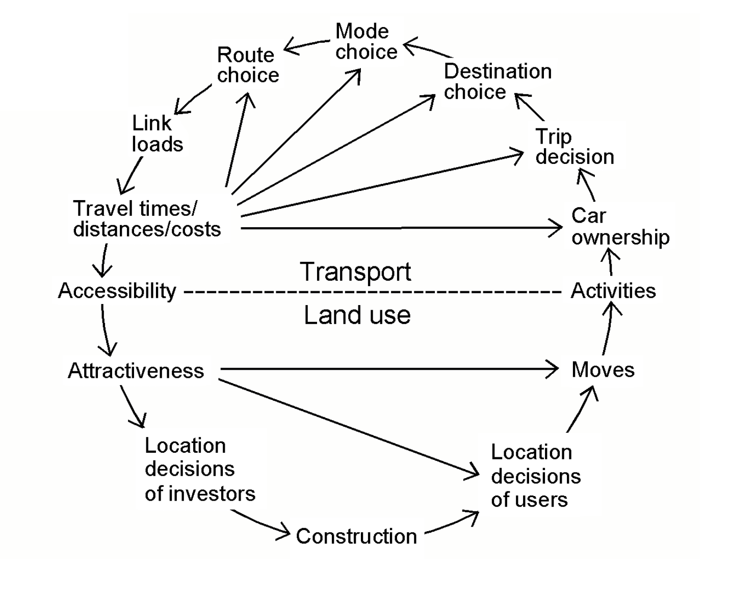
In an integrated land-use/transportation (LU-TR) model (which is a stack of structural models…2), there is a repetitive iteration between location choices and transportation choices (Wegener, 1994, 2004, 2021; Wegener, 1998). During each phase, the population chooses where to live and work. Then they choose how to commute and which route to take to work, which induces traffic congestion in the roadways. The congestion changes travel times, commuting speeds, and the level of accessibility at each location, so in the next round agents making location choices respond to this new layout (partially determined by choices other agents made). This yields a new spatial layout and a new set of transportation choices, etc., and this perpetual feedback loop allows land-use patterns and transport congestion to both be endogenous simulating into the future3.
In the 1950s first efforts were made in the USA to study the interrelationship between transport and the spatial development of cities systematically. Hansen (1959) demonstrated for Washington, DC that locations with good accessibility had a higher chance of being developed, and at a higher density, than remote locations (“How accessibility shapes land use”). The recognition that trip and location decisions co-determine each other and that therefore transport and land use planning needed to be co-ordinated, quickly spread among American planners, and the ‘land-use transport feedback cycle’ became a commonplace in the American planning literature. The set of relationships implied by this term can be briefly summarised as follows
- The distribution of land uses, such as residential, industrial or commercial, over the urban area determines the locations of human activities such as living, working, shopping, education or leisure.
- The distribution of human activities in space requires spatial interactions or trips in the transport system to overcome the distance between the locations of activities.
- The distribution of infrastructure in the transport system creates opportunities for spatial interactions and can be measured as accessibility.
- The distribution of accessibility in space co-determines location decisions and so results in changes of the land use system.
– Wegener (2004)
In this framework, you can modify many public policies, e.g. constraining land supply to discourage sprawl, adding a new toll lane to decrease congestion, or increasing a transit fare to raise revenue, and the modeling system predicts how people’s behavior adapts to the new (partial) equilibrium. There are two major benefits to this approach: first, at the micro-level, (and at each decision step) agents are represented by a series of behavioral models that should perform well out-of-sample, and second, the constant endogeneity allows for unexpected complexity and emergence patterns. A simulation based on parameters estimated from a residential location-choice model is just a Schelling model with more complicated (and realistic) equation that governs each agent’s behavior, and can yield similar emergence patterns (Benenson, 1998, 2004; Hatna & Benenson, 2012)
de Palma et al. (2007)
The model is estimated under a “random utility” framework using the UrbanSim2 software platform, in which a latent utility function is estimated based on the housing and neighborhood characteristics that define each unit (Foti & Waddell, n.d.). Household characteristics, such as income and household size enter into the model through interaction variables. This gives the discrete choice model with a conditional logit specification, as proposed by McFadden (1978), where the utility \(U\) provided by unit \(n\) for household \(i\) is
\[U = V_{ni} + \epsilon\]
where \(V_{ni}\) is linear-in-parameters of the form
\[V_{ni} =\alpha'Z_i + \beta'X_{ni}\]
with \(Z_i\) as a vector of dwelling attractiveness measures (housing characteristics like dwelling size, cost, accessibility, neighborhood composition, school quality, etc.) and \(X_{ni}\) as a vector of interaction terms of socio-demographic characteristics of household \(n\) with the attractiveness measures of dwelling \(i\). Assuming that \(\epsilon\) follows an extreme-value distribution, the probability \(P\) of household \(n\) choosing unit \(i\), is given by the multinomial logit model (Guo & Bhat, 2004)
\[P_{ni} = \frac{e^{V_{ni}}}{\sum_{i'}e^{V_{ni}}}\]
:::
Remember in the introduction when I said you do not let computer scientists or physicists make urban planning decisions? This is why.↩︎
By now, every modeler at every MPO in the country is rolling their eyes that I’ve characterized LU-TR models as anything other than hocus-pocus shaken inside a bag of bogus assumptions, then shamelessly ‘calibrated’ so the output matches control totals :)↩︎
This is why I continually stress the value of local computation in Chapter 14, because in integrated modeling (or just travel demand modeling) the cost/impedance of traveling along the network is constantly being changed as a function of the simulated land-use pattern (and how many other people are choosing to commute via highway, etc). Routing services from third parties are not capable of consuming these different networks, so they are effectively useless for serious scenario research (but by contrast, you can feed you own travel model to pandana
–that’s what it’s designed for)↩︎