13 Service Areas for Social Facilities

Code

import geopandas as gpd
import osmnx as ox
import pandana as pdna
from geosnap import DataStore
from geosnap.analyze import isochrones_from_gdf
from geosnap.io import get_acs, get_network_from_gdf

Code

%load_ext watermark
%watermark -a 'eli knaap' -v -d -u -p geopandas,geosnap
%load_ext autoreload
%autoreload 2

Author: eli knaap

Last updated: 2024-03-11

Python implementation: CPython
Python version       : 3.11.0
IPython version      : 8.18.1

geopandas: 0.14.2
geosnap  : 0.12.1.dev9+g3a1cb0f6de61.d20240110

Note this notebook requires osmnx

One way of thinking about isochrones is considering them as service areas. That is, given some travel budget (in time, distance, transit fare, etc), the isochrone represents the service area accessible within that budget.

Imagine we were interested in the service areas around social facilities in Syracuse

Code

datasets = DataStore()

Code

tracts = get_acs(datasets, msa_fips="45060", years=[2018], level="tract")

Code

facilities = ox.features.features_from_polygon(
    tracts.unary_union, {"amenity": "social_facility"}
)

Code

facilities = facilities[facilities.geometry.type == "Point"]

Code

tracts = tracts.to_crs(tracts.estimate_utm_crs())

Code

facilities = facilities.to_crs(tracts.crs)

Code

facilities.explore(style_kwds=dict(radius=4))

Make this Notebook Trusted to load map: File -> Trust Notebook

13.1 Walking Service Areas

Code

get_network_from_gdf?

Signature:
get_network_from_gdf(
    gdf,
    network_type='walk',
    twoway=False,
    add_travel_times=False,
    default_speeds=None,
)
Docstring:
Create a pandana.Network object from a geodataframe (via OSMnx graph).
Parameters
----------
gdf : geopandas.GeoDataFrame
    dataframe covering the study area of interest; Note the first step is to take
    the unary union of this dataframe, which is expensive, so large dataframes may
    be time-consuming. The network will inherit the CRS from this dataframe
network_type : str, {"all_private", "all", "bike", "drive", "drive_service", "walk"}
    the type of network to collect from OSM (passed to `osmnx.graph_from_polygon`)
    by default "walk"
twoway : bool, optional
    Whether to treat the pandana.Network as directed or undirected. For a directed network,
    use `twoway=False` (which is the default). For an undirected network (e.g. a
    walk network) where travel can flow in both directions, the network is more
    efficient when twoway=True but forces the impedance to be equal in both
    directions. This has implications for auto or multimodal
    networks where impedance is generally different depending on travel direction.
add_travel_times : bool, default=False
    whether to use posted travel times from OSM as the impedance measure (rather
    than network-distance). Speeds are based on max posted drive speeds, see
    <https://osmnx.readthedocs.io/en/stable/internals-reference.html#osmnx-speed-module>
    for more information.
default_speeds : dict, optional
    default speeds passed assumed when no data available on the OSM edge. Defaults
    to  {"residential": 35, "secondary": 50, "tertiary": 60}. Only considered if
    add_travel_times is True
Returns
-------
pandana.Network
    a pandana.Network object with node coordinates stored in the same system as the
    input geodataframe. If add_travel_times is True, the network impedance
    is travel time measured in seconds (assuming automobile travel speeds); else 
    the impedance is travel distance measured in meters
Raises
------
ImportError
    requires `osmnx`, raises if module not available
File:      ~/Dropbox/projects/geosnap/geosnap/io/networkio.py
Type:      function

Code

walk_net = get_network_from_gdf(tracts)

/Users/knaaptime/Dropbox/projects/geosnap/geosnap/io/networkio.py:71: UserWarning: GeoDataFrame is stored in coordinate system EPSG:32618 so the pandana.Network will also be stored in this system
  warn(

Generating contraction hierarchies with 10 threads.
Setting CH node vector of size 86033
Setting CH edge vector of size 226066
Range graph removed 216738 edges of 452132
. 10% . 20% . 30% . 40% . 50% . 60% . 70% . 80% . 90% . 100%

Code

isochrones_from_gdf?

Signature:
isochrones_from_gdf(
    origins,
    threshold,
    network,
    network_crs=None,
    reindex=True,
    hull='shapely',
    ratio=0.2,
    allow_holes=False,
    use_edges=True,
)
Docstring:
Create travel isochrones for several origins simultaneously
Parameters
----------
origins : geopandas.GeoDataFrame
    a geodataframe containing the locations of origin point features
threshold: float
    maximum travel cost to define the isochrone, measured in the same
    impedance units as edges_df in the pandana.Network object.
network : pandana.Network
    pandana Network instance for calculating the shortest path isochrone
    for each origin feature
network_crs : str, int, pyproj.CRS (optional)
    the coordinate system used to store x and y coordinates in the passed
    pandana network. If None, the network is assumed to be stored in the
    same CRS as the origins geodataframe
reindex : bool
    if True, use the dataframe index as the origin and destination IDs
    (rather than the node_ids of the pandana.Network). Default is True
hull : str, {'libpysal', 'shapely'}
    Which method to generate container polygons (concave hulls) for destination
    points. If 'libpysal', use `libpysal.cg.alpha_shape_auto` to create the
    concave hull, else if 'shapely', use  `shapely.concave_hull`.
    Default is libpysal
ratio : float
    ratio keyword passed to `shapely.concave_hull`. Only used if
    `hull='shapely'`. Default is 0.3
allow_holes : bool
    keyword passed to `shapely.concave_hull` governing  whether holes are
    allowed in the resulting polygon. Only used if `hull='shapely'`.
    Default is False.
use_edges: bool
    If true, use vertices from the Network.edge_df to make the polygon more
    accurate by adhering to roadways. Requires that the 'geometry' column be
    available on the Network.edges_df, most commonly by using
    `geosnap.io.get_network_from_gdf`
Returns
-------
GeoPandas.DataFrame
    polygon geometries with the isochrones for each origin point feature
File:      ~/Dropbox/projects/geosnap/geosnap/analyze/network.py
Type:      function

13.1.1 Comparing Hull algorithms

To create the service area, we need to bound the set of reachable intersections using some kind of polygon. The resolution of the service area is dependent on the resolution of the network (i.e. since geosnap and pandana do not interpolate along the road network, greater intersection density will result in a more well-defined polygon).

There are different bounding-polygon algorithms to choose from. The default is shapely’s concave_hull implementation, with the alpha_shape_auto algorithm from libpysal available as an alternative

Code

alpha = isochrones_from_gdf(
    facilities, network=walk_net, threshold=2000, hull="libpysal"
)

The alpha shape version of the concave hull is the most resource intensive because it tries to optimize the alpha parameter. This also makes it the slowest.

Code

m = alpha.explore()
facilities.explore(m=m, color="black", style_kwds=dict(radius=3))

Make this Notebook Trusted to load map: File -> Trust Notebook

Code

ch01 = isochrones_from_gdf(
    facilities, network=walk_net, threshold=2000, hull="shapely", ratio=0.1
)

The concave hull algorithm in shapely does not do automatic optimization, but requires setting a ratio parameter, with smaller values resulting in tighter bounding polygons. If the ratio parameter is set too low, the bounding polygon can be too tight

Code

m = ch01.explore()
facilities.explore(m=m, color="black", style_kwds=dict(radius=3))

Make this Notebook Trusted to load map: File -> Trust Notebook

Code

ch02 = isochrones_from_gdf(
    facilities, network=walk_net, threshold=2000, hull="shapely", ratio=0.2
)

Code

m = ch02.explore()
facilities.explore(m=m, color="black", style_kwds=dict(radius=3))

Make this Notebook Trusted to load map: File -> Trust Notebook

13.2 Driving Service Areas

Be very careful with driving times… There are lots of edges with no speed information (requiring us to make strong assumptions), and even at best, these represent free-flow conditions.

To get an automobile network, change network_type='drive' and add_travel_times=True

Code

drive_net = get_network_from_gdf(tracts, network_type="drive", add_travel_times=True)

/Users/knaaptime/Dropbox/projects/geosnap/geosnap/io/networkio.py:71: UserWarning: GeoDataFrame is stored in coordinate system EPSG:32618 so the pandana.Network will also be stored in this system
  warn(

Generating contraction hierarchies with 10 threads.
Setting CH node vector of size 24608
Setting CH edge vector of size 65928
Range graph removed 65088 edges of 131856
. 10% . 20% . 30% . 40% . 50% . 60% . 70% . 80% . 90% . 100%

When using travel-time based impedance, travel times are measured in seconds

Code

# 10 minute drive-shed

drive_chrone = isochrones_from_gdf(
    facilities, network=drive_net, threshold=600, ratio=0.1, allow_holes=False
)

Code

# look at only the first record

m = drive_chrone.iloc[[1]].explore()
facilities.iloc[[1]].explore(m=m, color="black", style_kwds=dict(radius=6))

/Users/knaaptime/mambaforge/envs/geosnap/lib/python3.11/site-packages/pyproj/transformer.py:820: DeprecationWarning: Conversion of an array with ndim > 0 to a scalar is deprecated, and will error in future. Ensure you extract a single element from your array before performing this operation. (Deprecated NumPy 1.25.)
  return self._transformer._transform_point(

Make this Notebook Trusted to load map: File -> Trust Notebook

Code

drive_net.edges_df

	from	to	travel_time	geometry
0	211905525	212550604	40.6	LINESTRING (451007.906 4731874.375, 450991.739...
1	211905525	6291988938	166.9	LINESTRING (451007.906 4731874.375, 450989.152...
2	212028019	212827209	55.3	LINESTRING (426356.190 4737964.394, 426356.358...
3	212533433	212533484	4.4	LINESTRING (429887.965 4753965.714, 429886.570...
4	212533433	212533444	12.6	LINESTRING (429887.965 4753965.714, 429814.773...
...	...	...	...	...
65923	10917595296	213148992	19.6	LINESTRING (404376.996 4832069.741, 404376.929...
65924	10942234832	213009542	24.0	LINESTRING (397377.555 4819328.544, 397372.182...
65925	10942234832	213045439	4.3	LINESTRING (397377.555 4819328.544, 397381.484...
65926	10942234832	213177620	34.8	LINESTRING (397377.555 4819328.544, 397373.513...
65927	11012738718	212991426	4.3	LINESTRING (378806.020 4814057.760, 378820.010...

65928 rows × 4 columns

Remember also this is directed travel. These isochrones represent the area reachable from each social service provider; they do not necesssarily represent the origins who can reach the provider within a 10 minute drive. That is, drive networks are directed (and usually asymmetric).

13.3 Comparing with Routing Servers

This notebook only runs with routingpy, which is incompatible with shapely 2 at the moment

Here, I’ve setup an instance of the valhalla routing server on a cloud server. It’s actually pretty easy–everything is in docker, but you won’t be able to follow along unless you setup your own server and edit the URL below accordingly

Code

import geopandas as gpd
import pandas as pd
from geosnap import DataStore
from geosnap import analyze as gaz
from geosnap import io as gio
from routingpy import Valhalla
from shapely.geometry import Polygon


datasets = DataStore()

---------------------------------------------------------------------------

ModuleNotFoundError                       Traceback (most recent call last)

Cell In[1], line 6

      4 from geosnap import analyze as gaz

      5 from geosnap import io as gio

----> 6 from routingpy import Valhalla

      7 from shapely.geometry import Polygon

     10 datasets = DataStore()



ModuleNotFoundError: No module named 'routingpy'

Often, you need routing, or travel time matrices, or isochrones for a place, but commercial or cloud-based solutions are not an option. For example if:

you have sensitive data that can’t be sent to remote servers
you have a massive dataset and end up being rate-limited (and/or hitting a paywall)
you need control over how the network is structured and parameterized (for example if you are testing different potential transit scenarios)

All of those cases require more control over the routing than web services can provide, which leaves two strong options for local computation.

Code

sd = gio.get_acs(datasets, county_fips='06073', years=[2019], level='tract')
sd = sd[sd.n_total_pop >0]

Code

sd.plot()

<AxesSubplot:>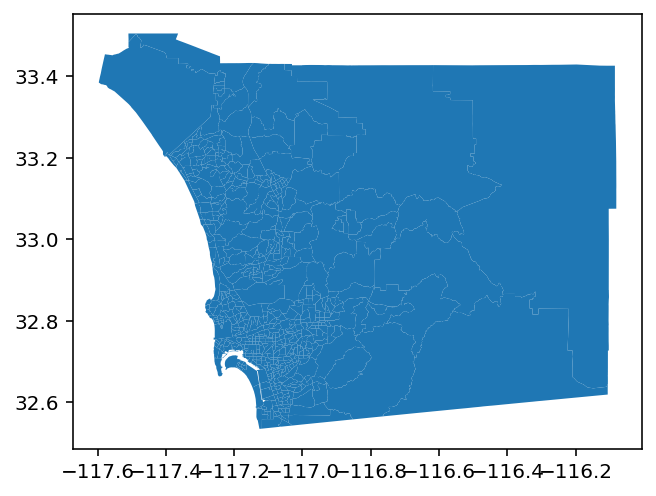

Code

# grab 10 observations
sdsub = sd.head(10)

Code

coords = list(zip(sdsub.geometry.centroid.get_coordinates().x.tolist(), sdsub.geometry.centroid.y))

UserWarning: Geometry is in a geographic CRS. Results from 'centroid' are likely incorrect. Use 'GeoSeries.to_crs()' to re-project geometries to a projected CRS before this operation.

  coords = list(zip(sdsub.geometry.centroid.get_coordinates().x.tolist(), sdsub.geometry.centroid.y))
<ipython-input-5-9c471eba5560>:1: UserWarning: Geometry is in a geographic CRS. Results from 'centroid' are likely incorrect. Use 'GeoSeries.to_crs()' to re-project geometries to a projected CRS before this operation.

  coords = list(zip(sdsub.geometry.centroid.get_coordinates().x.tolist(), sdsub.geometry.centroid.y))

13.4 Testing the valhalla routing engine

One is to setup a locally-hosted open-source routing engine and query that server instead of a commercial server (as you would do with a geocoding service). This is nice because they are highly performant, but the drawbacksa are: - can be a little difficult to setup and maintain, or ingest new data - can take a ton of compute/storage/memory resources, so may require your own “server” - can make the work unreproducible in many contexts, because anyone running the code also needs access to the local server. We use tailscale to share compute resources, but that adds a small layer of complexity

Code

# no trailing slash, api_key is not necessary
# you need to be connected to tailscale for this to work

client = Valhalla(base_url="http://cogs-research:8002", timeout=6000)

Code

client.isochrones.ex

Init signature: client.Waypoint(position, **kwargs)
Docstring:     
Constructs a waypoint with additional information or constraints.
Refer to Valhalla's documentation for details: https://github.com/valhalla/valhalla/blob/master/docs/api/turn-by-turn/api-reference.md#locations
Use ``kwargs`` to spedify options, make sure the value is proper for each option.
Example:
>>> waypoint = Valhalla.WayPoint(position=[8.15315, 52.53151], type='through', heading=120, heading_tolerance=10, minimum_reachability=10, radius=400)
>>> route = Valhalla('http://localhost').directions(locations=[[[8.58232, 51.57234]], waypoint, [7.15315, 53.632415]])
File:           ~/mambaforge/envs/geosnap/lib/python3.9/site-packages/routingpy/routers/valhalla.py
Type:           type
Subclasses:

Code

# valhalla can do one origin at a time, so only pass the first

test_isos = client.isochrones(coords[0], 'pedestrian', intervals=[1000,1500,2000,2500], interval_type='distance')

Code

# turn the json response into gdfs
def gdf_from_routingpy(isos):
    polys = [Polygon(i['geometry']['coordinates']) for i in isos.raw['features']]
    gdf = gpd.GeoDataFrame(geometry=polys, crs=4326)
    return gdf

Code

gdf = gdf_from_routingpy(test_isos)

Code

gdf.explore()

Make this Notebook Trusted to load map: File -> Trust Notebook

13.4.1 How do these compare to the geosnap isos?

Code

import pandana as pdna
sdnet = pdna.Network.from_hdf5("/Users/knaaptime/Dropbox/projects/geosnap_data/metro_networks_8k/41740.h5")

Code

gisos = pd.concat([gaz.isochrones(gpd.GeoDataFrame(sdsub.iloc[0].to_frame().T), threshold=t, network=sdnet) for t in [1000,1500,2000,2500]])

Code

gisos.explore()

Make this Notebook Trusted to load map: File -> Trust Notebook

Code

gdf.explore()

Make this Notebook Trusted to load map: File -> Trust Notebook

The isochrones are pretty consistent, so i think the differences between the two are:

valhalla uses a tighter alpha shape
it can do that because it interpolates nodes distance along the road network, rather than requiring you to hit an actual intersection (as we assume in the pandana/geosnap approach

13.4.1.1 Comparing 2500m

Code

m = gdf.head(1).explore()

Code

gisos[gisos['distance']==2500].explore(m=m)

13.5 Travel Time matrix

Code

sd.shape[0]**2

Code

client.matrix?

Signature:
client.matrix(
    locations,
    profile,
    sources=None,
    destinations=None,
    preference=None,
    options=None,
    avoid_locations=None,
    avoid_polygons=None,
    units=None,
    id=None,
    dry_run=None,
)
Docstring:
Gets travel distance and time for a matrix of origins and destinations.
For more information, visit https://github.com/valhalla/valhalla/blob/master/docs/api/matrix/api-reference.md.
Use ``kwargs`` for any missing ``matrix`` request options.
:param locations: Multiple pairs of lng/lat values.
:type locations: list of list
:param profile: Specifies the mode of transport to use when calculating
    matrices. One of ["auto", "bicycle", "multimodal", "pedestrian".
:type profile: str
:param sources: A list of indices that refer to the list of locations
    (starting with 0). If not passed, all indices are considered.
:type sources: list of int
:param destinations: A list of indices that refer to the list of locations
    (starting with 0). If not passed, all indices are considered.
:type destinations: list of int
:param str preference: Convenience argument to set the cost metric, one of ['shortest', 'fastest']. Note,
    that shortest is not guaranteed to be absolute shortest for motor vehicle profiles. It's called ``preference``
    to be inline with the already existing parameter in the ORS adapter.
:param options: Profiles can have several options that can be adjusted to develop the route path,
    as well as for estimating time along the path. Only specify the actual options dict, the profile
    will be filled automatically. For more information, visit:
    https://github.com/valhalla/valhalla/blob/master/docs/api/turn-by-turn/api-reference.md#costing-options
:type options: dict
:param avoid_locations: A set of locations to exclude or avoid within a route.
    Specified as a list of coordinates, similar to coordinates object.
:type avoid_locations: list of list
:param List[List[List[float]]] avoid_polygons: One or multiple exterior rings of polygons in the form of nested
    JSON arrays, e.g. [[[lon1, lat1], [lon2,lat2]],[[lon1,lat1],[lon2,lat2]]]. Roads intersecting these rings
    will be avoided during path finding. If you only need to avoid a few specific roads, it's much more
    efficient to use avoid_locations. Valhalla will close open rings (i.e. copy the first coordingate to the
    last position).
:param units: Distance units for output. One of ['mi', 'km']. Default km.
:type units: str
:param id: Name your route request. If id is specified, the naming will be sent through to the response.
:type id: str
:param dry_run: Print URL and parameters without sending the request.
:param dry_run: bool
:returns: A matrix from the specified sources and destinations.
:rtype: :class:`routingpy.matrix.Matrix`
    
File:      ~/mambaforge/envs/geosnap/lib/python3.9/site-packages/routingpy/routers/valhalla.py
Type:      method

Code

# pairwise matrix for all tract centroids in SD county
coords = list(zip(sd.geometry.centroid.get_coordinates().x.tolist(), sd.geometry.centroid.y))

UserWarning: Geometry is in a geographic CRS. Results from 'centroid' are likely incorrect. Use 'GeoSeries.to_crs()' to re-project geometries to a projected CRS before this operation.

  coords = list(zip(sd.geometry.centroid.get_coordinates().x.tolist(), sd.geometry.centroid.y))
<ipython-input-17-e7ac3013bf3d>:2: UserWarning: Geometry is in a geographic CRS. Results from 'centroid' are likely incorrect. Use 'GeoSeries.to_crs()' to re-project geometries to a projected CRS before this operation.

  coords = list(zip(sd.geometry.centroid.get_coordinates().x.tolist(), sd.geometry.centroid.y))

:::