21 The Dimensions of Residential Segregation

A seminal contribution in segregation measurement is given by Massey & Denton (1988) who were the first to examine quantitatively the wide variety of segregation indexing strategies and the information each provides. Their paper is important first because of the sheer volume of work: in the late 80s, it was seriously laborious to gather data for a large number of metropolitan regions and compute a dozen segregation indices in each one; the paper’s second major contribution is the way it helped clarify the relationships among various indices that had been proposed over the years.

Like personality theory and item-response theory in psychology, Massey and Denton proposed that there were multiple ways to measure segregation that capture different concepts of the term (i.e. unevenness versus clustering)–but there probably are not 20 different concepts like there are indices in use. Instead, those two dozen indices are different ways of capturing the five or so dimensions of segregation that really exist (they argue). This was a dramatic step forward in understanding what we’re actually measuring when we study residential segregation.

Code

import os

import geopandas as gpd
import matplotlib.pyplot as plt
import networkx as nx
import pandas as pd
import seaborn as sns
from factor_analyzer import FactorAnalyzer
from geosnap import DataStore
from geosnap import io as gio
from networkx.drawing.nx_agraph import graphviz_layout
from segregation.batch import batch_compute_multigroup, batch_compute_singlegroup
from sklearn.cluster import AffinityPropagation, AgglomerativeClustering, KMeans
from sklearn.metrics import silhouette_score

%load_ext watermark
%watermark -a 'eli knaap' -iv

OMP: Info #276: omp_set_nested routine deprecated, please use omp_set_max_active_levels instead.

Author: eli knaap

networkx  : 3.0
geopandas : 0.14.1
geosnap   : 0.12.0
seaborn   : 0.12.2
matplotlib: 3.4.3
pandas    : 1.5.3

Code

sns.set_context('notebook')

Following Massey & Denton (1988) (also MASSEY et al. (1996) and Massey (2012)) we can look at dimensionality in segregation measures by computing two-group indices for Black, Hispanic, and Asian groups (vs white) for every metro region in the country. Here we will use the 2021 ACS data at the blockgroup level, and use a 2km radius for computing generalized spatial measures, which helps account for heterogeneity in BG size

Code

multi_groups = [
    "n_nonhisp_white_persons",
    "n_nonhisp_black_persons",
    "n_hispanic_persons",
    "n_asian_persons",
]

Code

singles = ["n_nonhisp_black_persons", "n_hispanic_persons", "n_asian_persons"]

Code

datasets = DataStore()

Code

msas = datasets.msas()

Code

msas = msas[msas["type"].str.startswith("Metro")]  # only metros not micros

Code

msa_fips = msas.geoid.values

21.1 Two-Group Measures

Code

for group in singles:
    if not os.path.exists(f"../data/{group}_measures.csv"):
        dfs = []
        for metro in msa_fips:
            try:
                # get blockgroup-level data for the MSA
                df = gio.get_acs(datasets, msa_fips=metro, level="bg", years=[2021])
                # create a temporary 'total' population of white/other
                df["temp_total"] = df[group] + df["n_nonhisp_white_persons"]
                df = df.dropna(subset=["geometry"]).to_crs(df.estimate_utm_crs())
                # compute all seg measures with a 2km neighborhood
                seg = batch_compute_singlegroup(
                    df, group_pop_var=group, total_pop_var="temp_total", distance=2000
                )
                dfs.append(seg.Statistic.rename(metro))
            except Exception as e:  # PR will fail
                print(e)
                df = None
                pass
        results = pd.concat(dfs, axis=1).T
        results.to_csv(f"../data/{group}_measures.csv")

Code

results = pd.concat(
    [pd.read_csv(f"../data/{group}_measures.csv", index_col=0) for group in singles]
)

Code

results

	AbsoluteCentralization	AbsoluteClustering	AbsoluteConcentration	Atkinson	BiasCorrectedDissim	BoundarySpatialDissim	ConProf	CorrelationR	Delta	DensityCorrectedDissim	...	MinMax	ModifiedDissim	ModifiedGini	PARDissim	RelativeCentralization	RelativeClustering	RelativeConcentration	SpatialDissim	SpatialProxProf	SpatialProximity
10180	0.9042	0.2060	0.9826	0.1854	0.2700	0.4386	0.0912	0.0711	0.9389	0.2354	...	0.4268	0.2526	0.3842	0.5578	0.2732	2.8646	0.8783	0.4294	0.3103	1.1767
10420	0.6662	0.1589	0.9315	0.3920	0.5184	0.5253	0.3129	0.2655	0.7895	0.2338	...	0.6831	0.5113	0.6634	0.6148	0.3112	1.2762	0.6891	0.5175	0.3230	1.1463
10500	0.7307	0.1498	0.7150	0.4416	0.5449	0.3733	0.6500	0.3603	0.7642	0.3928	...	0.7058	0.5366	0.7039	0.5224	0.3250	-0.3211	0.6843	0.3549	1.2321	1.1838
10740	0.9356	0.0814	0.9715	0.1645	0.3076	NaN	0.0594	0.0435	0.9527	0.3065	...	0.4720	0.2865	0.4018	0.5727	0.1409	1.8258	0.5618	0.5001	0.1721	1.0728
10780	0.8175	0.2732	0.8932	0.4960	0.5688	0.4437	0.4854	0.3902	0.8486	0.3596	...	0.7253	0.5609	0.7229	0.6129	0.4747	0.6398	0.7614	0.4309	0.6865	1.2401
...	...	...	...	...	...	...	...	...	...	...	...	...	...	...	...	...	...	...	...	...	...
49420	0.8819	0.1295	0.9884	0.3293	0.4473	0.6066	0.0821	0.0729	0.9325	0.4331	...	0.6193	0.4248	0.5729	0.6500	0.3188	5.3510	0.7655	0.6027	0.1564	1.1197
49620	0.5282	0.0403	0.9106	0.2805	0.3691	0.6393	0.0256	0.0222	0.8133	0.3260	...	0.5422	0.3401	0.4777	0.6631	0.2947	3.7648	0.4683	0.6369	0.0929	1.0365
49660	0.5693	0.0525	0.9268	0.4412	0.4899	0.7501	0.0290	0.0272	0.8686	0.4154	...	0.6617	0.4498	0.6161	0.7616	0.1188	9.3811	0.4258	0.7487	0.0423	1.0503
49700	0.8876	0.2421	0.9240	0.1872	0.3156	0.3531	0.1736	0.1205	0.8744	0.2860	...	0.4801	0.3039	0.4390	0.4757	0.1219	1.8433	0.7137	0.3512	0.3706	1.1877
49740	0.9686	0.0656	0.9851	0.2637	0.3569	0.5350	0.0465	0.0397	0.9611	0.3272	...	0.5278	0.3238	0.4655	0.5713	0.2100	2.1184	0.7531	0.5346	0.1533	1.0529

906 rows × 27 columns

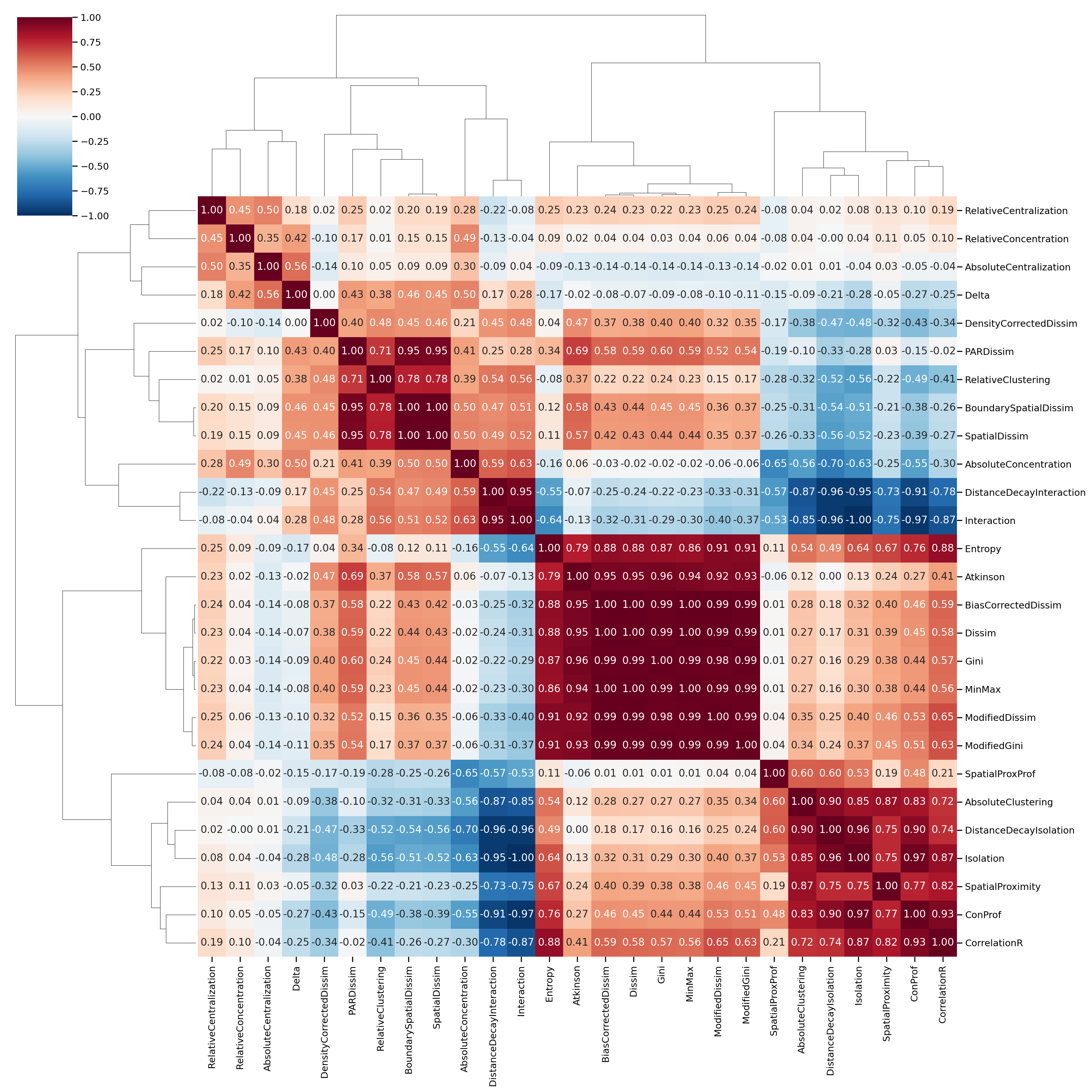
One of the easiest ways to understand the dimensionality in the dataset is a heatmap of the variable correlation matrix

Code

sns.clustermap(results.corr(), cmap="RdBu_r", annot=True, fmt=".2f", figsize=(18, 18))

The large contiguous blocks are groups of variables that are highly intercorrelated, and capture largely the “same thing”. Whether the underlying concept being measured is a factor or a component is a matter of debate. In the segregation context, these different indices are probably better treated as components that capture slightly different measurements of the same construct, rather than manifest outcomes of some underlying latent process of, e.g. “unevenness segregation”. That is, the Gini and Dissimilarity indices are probably different ways of measuring ‘unevenness’, as opposed to a social process of unevenness that manifests as these two different variables, “gini” and “dissimilarity”… As Rees (1971) describes, factor analysis applied to urban data more often adopts the alternative: “more modest is the claim that components or factors represent concise descriptions of patterns of associations of attributes across observations.”

All the same, the Massey and Denton approach that treats dimensions as factors is a useful way of tackling the problem, and we can adopt the factor view to recreate their analysis.

Code

# boundary spatial dissim gives a few NaNs (from islands, i think)
results[results.isna().any(axis=1)]

	AbsoluteCentralization	AbsoluteClustering	AbsoluteConcentration	Atkinson	BiasCorrectedDissim	BoundarySpatialDissim	ConProf	CorrelationR	Delta	DensityCorrectedDissim	...	MinMax	ModifiedDissim	ModifiedGini	PARDissim	RelativeCentralization	RelativeClustering	RelativeConcentration	SpatialDissim	SpatialProxProf	SpatialProximity
10740	0.9356	0.0814	0.9715	0.1645	0.3076	NaN	0.0594	0.0435	0.9527	0.3065	...	0.4720	0.2865	0.4018	0.5727	0.1409	1.8258	0.5618	0.5001	0.1721	1.0728
19740	0.9328	0.1731	0.9827	0.3762	0.5149	NaN	0.2018	0.1796	0.9405	0.2549	...	0.6799	0.5064	0.6606	0.6771	0.2575	3.0679	0.8064	0.6038	0.2126	1.1544
31080	0.6884	0.3311	0.8999	0.5457	0.6303	NaN	0.5386	0.4672	0.8390	0.1353	...	0.7733	0.6258	0.7783	0.6785	0.4760	1.5706	0.5242	0.5632	0.2764	1.2815
41860	0.6508	0.2321	0.9147	0.3107	0.4546	NaN	0.2752	0.2239	0.8533	0.1484	...	0.6251	0.4487	0.6008	0.6384	0.2699	1.5507	0.5507	0.5229	0.2824	1.2089
46520	0.5012	0.1874	0.8429	0.1702	0.3156	NaN	0.0887	0.0632	0.9166	0.3018	...	0.4809	0.2997	0.4174	0.5690	0.1578	2.1190	0.0153	0.4563	0.2459	1.1352
10740	0.9053	0.2310	0.4648	0.1642	0.3134	NaN	0.3791	0.1447	0.9018	0.1753	...	0.4775	0.3060	0.4247	0.3508	0.0018	0.0099	0.1296	0.2119	1.3006	1.1014
19740	0.9141	0.1961	0.9085	0.2367	0.4107	NaN	0.3203	0.2095	0.8924	0.1452	...	0.5823	0.4050	0.5317	0.4850	0.1741	0.6973	0.7232	0.3591	0.4424	1.1587
31080	0.6802	0.4191	0.5952	0.4549	0.5736	NaN	0.6825	0.3785	0.7699	0.0560	...	0.7291	0.5705	0.7289	0.5995	0.3857	-0.0737	0.5477	0.4795	1.6263	1.2418
41860	0.5482	0.2895	0.7566	0.2418	0.4098	NaN	0.3707	0.2250	0.8013	0.0920	...	0.5814	0.4053	0.5309	0.5044	0.0370	0.4790	0.4541	0.3606	0.6331	1.2095
46520	0.4444	0.2179	0.7003	0.0967	0.2434	NaN	0.1952	0.0888	0.8694	0.2423	...	0.3919	0.2327	0.3282	0.3971	0.0988	0.0083	0.2940	0.1780	0.6497	1.1100
10740	0.9463	0.1239	0.9595	0.1743	0.3095	NaN	0.0607	0.0469	0.9506	0.3085	...	0.4742	0.2886	0.4098	0.5575	0.1453	3.3333	0.3723	0.5034	0.1588	1.1120
19740	0.8973	0.0722	0.9774	0.1465	0.3089	NaN	0.0589	0.0427	0.9069	0.3032	...	0.4727	0.2942	0.4045	0.4932	0.0220	1.5757	0.6993	0.4285	0.1438	1.0611
31080	0.6385	0.3197	0.7962	0.2809	0.4430	NaN	0.3979	0.2562	0.7646	0.1187	...	0.6141	0.4378	0.5790	0.4897	0.2828	0.4117	0.5438	0.3313	0.6188	1.2099
41860	0.6035	0.2965	0.6825	0.1650	0.3250	NaN	0.3017	0.1534	0.7944	0.0915	...	0.4906	0.3205	0.4439	0.4698	0.0651	0.3843	0.3626	0.3233	0.7680	1.1867
46520	0.4950	0.3607	0.4543	0.1356	0.2451	NaN	0.3491	0.0981	0.8743	0.1299	...	0.3939	0.2381	0.3625	0.4694	0.2371	-0.3543	0.5614	0.3010	2.5577	1.1778

15 rows × 27 columns

Affinity propagation is a clustering algorithm where k is endogenous. If we fit a clusterer to the correlation matrix of segregation indices, we’re looking for groups of variables that capture the same dimension. This works for our purposes here because we don’t really care about the factor loadings or measuring the latent construct per se (the segregation measures themselves are preferable for that). Instead, we’re asking whether these indices are providing unique information, and how many unique dimensions should we consider?

Since cluster assignments are discrete, and we think of cluster assignments as ‘best’ when they are unambiguous (i.e. clusters are well-separated and each observation belongs to only one cluster), this is like treating the dimensions as orthogonal in factor analysis… If we think the factors are correlated (oblique rotated), then the clusters wouldn’t be well-separated.

Code

ap = AffinityPropagation().fit_predict(results.corr())

Code

ap = pd.Series(dict(zip(results.columns.values, ap)), name="Index Type")

Code

ap.nunique()

Code

silhouette_score(results.corr(), ap)

0.6031665663470883

Code

ap.sort_values()

SpatialProximity            0
SpatialProxProf             0
DistanceDecayIsolation      0
CorrelationR                0
ConProf                     0
Isolation                   0
AbsoluteClustering          0
RelativeClustering          1
SpatialDissim               1
DensityCorrectedDissim      1
BoundarySpatialDissim       1
PARDissim                   1
Interaction                 2
DistanceDecayInteraction    2
AbsoluteConcentration       2
ModifiedGini                3
ModifiedDissim              3
Entropy                     3
Gini                        3
Dissim                      3
BiasCorrectedDissim         3
Atkinson                    3
MinMax                      3
Delta                       4
RelativeCentralization      4
RelativeConcentration       4
AbsoluteCentralization      4
Name: Index Type, dtype: int64

Code

clust_labels = AgglomerativeClustering(n_clusters=5).fit_predict(results.corr())

Code

clust_labels = pd.Series(dict(zip(results.columns.values, clust_labels)))

Code

clust_labels.sort_values()

SpatialProximity            0
AbsoluteClustering          0
ConProf                     0
CorrelationR                0
Isolation                   0
DistanceDecayIsolation      0
SpatialProxProf             0
AbsoluteConcentration       1
Interaction                 1
DistanceDecayInteraction    1
ModifiedGini                2
ModifiedDissim              2
MinMax                      2
Gini                        2
Entropy                     2
BiasCorrectedDissim         2
Atkinson                    2
Dissim                      2
Delta                       3
RelativeCentralization      3
RelativeConcentration       3
AbsoluteCentralization      3
DensityCorrectedDissim      4
BoundarySpatialDissim       4
PARDissim                   4
RelativeClustering          4
SpatialDissim               4
dtype: int64

Code

silhouette_score(results.corr(), clust_labels)

0.6031665663470883

The interesting thing is how well these results map onto Massey and Denton’s originals, despite the idea that clustering and exposure make more sense collapsed into a single category (that concept seems even more pronounced in these results, since isolation and interaction are basically inverses, but end up in different categories)

Code

clust_labels = AgglomerativeClustering(n_clusters=3).fit_predict(results.corr())

Code

clust_labels = pd.Series(dict(zip(results.columns.values, clust_labels)))

Code

silhouette_score(results.corr(), clust_labels)

0.5582547485763226

Code

clust_labels.sort_values()

AbsoluteCentralization      0
SpatialDissim               0
AbsoluteConcentration       0
RelativeConcentration       0
RelativeClustering          0
BoundarySpatialDissim       0
RelativeCentralization      0
PARDissim                   0
Delta                       0
DensityCorrectedDissim      0
DistanceDecayInteraction    0
Interaction                 0
Isolation                   1
SpatialProximity            1
DistanceDecayIsolation      1
CorrelationR                1
ConProf                     1
AbsoluteClustering          1
SpatialProxProf             1
Gini                        2
Dissim                      2
MinMax                      2
ModifiedDissim              2
ModifiedGini                2
BiasCorrectedDissim         2
Atkinson                    2
Entropy                     2
dtype: int64

Code

klabels = KMeans(n_clusters=5).fit_predict(results.corr())

/Users/knaaptime/mambaforge/envs/urban_analysis/lib/python3.10/site-packages/sklearn/cluster/_kmeans.py:870: FutureWarning: The default value of `n_init` will change from 10 to 'auto' in 1.4. Set the value of `n_init` explicitly to suppress the warning
  warnings.warn(

Code

klabels = pd.Series(dict(zip(results.columns.values, klabels)))

Code

silhouette_score(results.corr(), klabels.values)

0.6031665663470883

The clustering algorithms are all really stable in their assignments. When you tune hierarchical and kmeans using the optimal silhouette score, they agree on the exact assignments in the 5 cluster solution

21.2 Factor Analysis

from the psych docs https://personality-project.org/r/psych-manual.pdf:

Factor analysis is an attempt to approximate a correlation or covariance matrix with one of lesser rank. The basic model is that nRn ≈n FkkF 0 n + U 2 where k is much less than n. There are many ways to do factor analysis, and maximum likelihood procedures are probably the most commonly preferred (see factanal ). The existence of uniquenesses is what distinguishes factor analysis from principal components analysis (e.g., principal). If variables are thought to represent a “true” or latent part then factor analysis provides an estimate of the correlations with the latent factor(s) representing the data. If variables are thought to be measured without error, then principal components provides the most parsimonious description of the data. Factor loadings will be smaller than component loadings for the later reflect unique error in each variable. The off diagonal residuals for a factor solution will be superior (smaller) that of a component model. Factor loadings can be thought of as the asymptotic component loadings as the number of variables loading on each factor increases

Code

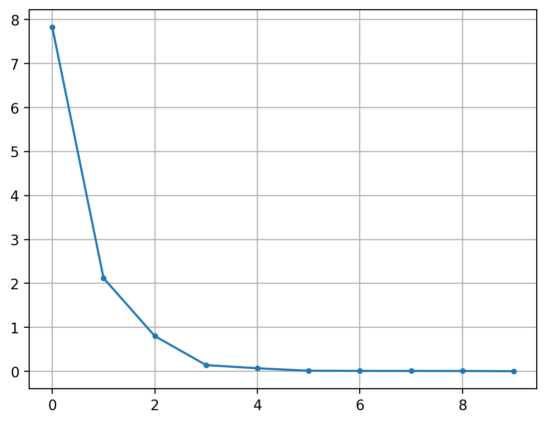
# first look for n_factors)
fa = FactorAnalyzer(rotation="oblimin", n_factors=results.shape[1])

Code

fa.fit(results.fillna(0))

FactorAnalyzer(n_factors=27, rotation='oblimin', rotation_kwargs={})

In a Jupyter environment, please rerun this cell to show the HTML representation or trust the notebook.
On GitHub, the HTML representation is unable to render, please try loading this page with nbviewer.org.

Code

ev, v = fa.get_eigenvalues()

Code

ev = pd.Series(ev)

Code

ev.iloc[:10].plot(grid=True, style=".-", figsize=(6,6))

The scree plot suggests an albow at about 3, maybe 4. Revelle says do not use the eigenvalue >1 rule to determine n_factors

Code

from scipy.stats import zscore

Code

fa = FactorAnalyzer(rotation="oblimin", n_factors=5)
fa.fit(results)

FactorAnalyzer(n_factors=5, rotation='oblimin', rotation_kwargs={})

Code

factors = pd.DataFrame.from_records(
    fa.loadings_, index=results.columns, columns=["F1", "F2", "F3", "F4", "F5"]
)

loadings less than .1 are considered unimportant (R and others suppress them). Revelle says ignore less than .3.

We will follow Massey and Denton and the clustering results above, and shoot for 5 factors

Code

factors = factors.mask(factors < 0.3)

Code

factors

	F1	F2	F3	F4	F5
AbsoluteCentralization	NaN	NaN	NaN	NaN	0.717832
AbsoluteClustering	NaN	NaN	0.695828	0.475336	NaN
AbsoluteConcentration	NaN	NaN	NaN	NaN	0.314571
Atkinson	0.927950	NaN	NaN	NaN	NaN
BiasCorrectedDissim	0.975286	NaN	NaN	NaN	NaN
BoundarySpatialDissim	NaN	0.866075	NaN	NaN	NaN
ConProf	0.329183	NaN	0.560560	NaN	NaN
CorrelationR	0.481336	NaN	0.670719	NaN	NaN
Delta	NaN	0.626410	NaN	NaN	0.424750
DensityCorrectedDissim	0.526844	NaN	NaN	NaN	NaN
Dissim	0.974563	NaN	NaN	NaN	NaN
DistanceDecayInteraction	NaN	NaN	NaN	NaN	NaN
DistanceDecayIsolation	NaN	NaN	0.526268	0.528260	NaN
Entropy	0.815438	NaN	0.377583	NaN	NaN
Gini	0.971297	NaN	NaN	NaN	NaN
Interaction	NaN	NaN	NaN	NaN	NaN
Isolation	NaN	NaN	0.516079	0.360120	NaN
MinMax	0.974450	NaN	NaN	NaN	NaN
ModifiedDissim	0.968980	NaN	NaN	NaN	NaN
ModifiedGini	0.972560	NaN	NaN	NaN	NaN
PARDissim	0.311544	0.859431	NaN	NaN	NaN
RelativeCentralization	0.314008	NaN	NaN	NaN	0.725198
RelativeClustering	NaN	0.780695	NaN	NaN	NaN
RelativeConcentration	NaN	NaN	NaN	NaN	0.588542
SpatialDissim	NaN	0.857307	NaN	NaN	NaN
SpatialProxProf	NaN	NaN	NaN	0.864273	NaN
SpatialProximity	NaN	NaN	0.876189	NaN	NaN

The latent factors are on the columns and the loadings for each variable are on the rows

Code

for f in factors.columns:
    print(f"{f}:\n",factors.dropna(subset=[f])[f],"\n")

F1:
 Atkinson                  0.927950
BiasCorrectedDissim       0.975286
ConProf                   0.329183
CorrelationR              0.481336
DensityCorrectedDissim    0.526844
Dissim                    0.974563
Entropy                   0.815438
Gini                      0.971297
MinMax                    0.974450
ModifiedDissim            0.968980
ModifiedGini              0.972560
PARDissim                 0.311544
RelativeCentralization    0.314008
Name: F1, dtype: float64 

F2:
 BoundarySpatialDissim    0.866075
Delta                    0.626410
PARDissim                0.859431
RelativeClustering       0.780695
SpatialDissim            0.857307
Name: F2, dtype: float64 

F3:
 AbsoluteClustering        0.695828
ConProf                   0.560560
CorrelationR              0.670719
DistanceDecayIsolation    0.526268
Entropy                   0.377583
Isolation                 0.516079
SpatialProximity          0.876189
Name: F3, dtype: float64 

F4:
 AbsoluteClustering        0.475336
DistanceDecayIsolation    0.528260
Isolation                 0.360120
SpatialProxProf           0.864273
Name: F4, dtype: float64 

F5:
 AbsoluteCentralization    0.717832
AbsoluteConcentration     0.314571
Delta                     0.424750
RelativeCentralization    0.725198
RelativeConcentration     0.588542
Name: F5, dtype: float64

first factor loads heavily on dissim, gini, minmax, entropy (evenness)

f2 loads on isolation and clustering, proximity (clustering)

this solution looks like there’s probably closer to 3 factors… 3 and 4 are almost collinear

Code

fa.phi_

array([[ 1.        ,  0.22549582,  0.04086467,  0.11374999,  0.31756587],
       [ 0.22549582,  1.        ,  0.09986776, -0.3944805 , -0.363344  ],
       [ 0.04086467,  0.09986776,  1.        , -0.03852471,  0.26115788],
       [ 0.11374999, -0.3944805 , -0.03852471,  1.        ,  0.46093543],
       [ 0.31756587, -0.363344  ,  0.26115788,  0.46093543,  1.        ]])

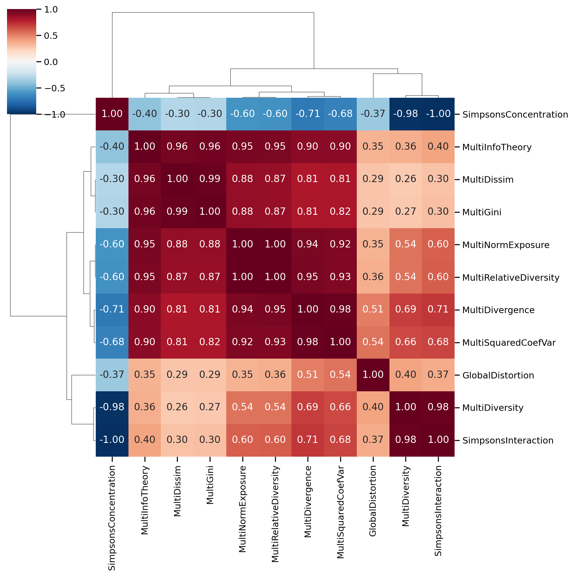
the phi_ attribute stores the factor correlation matrix, which looks pretty reasonable here. There is some correlation among the factors (as expected, since we used an oblique transform, intentionally), but nothing that looks overlapping. In other words, while the factors look like they may be related, each one is capturing unique information as well

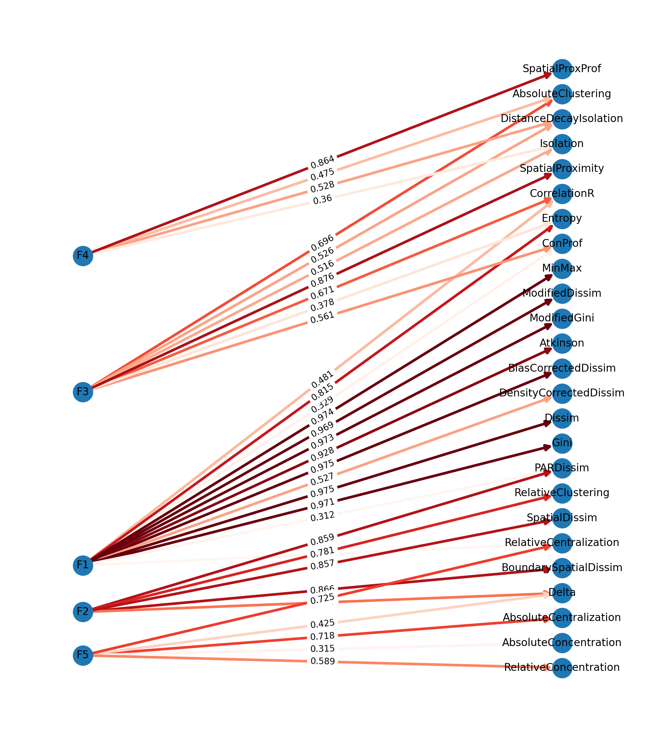
The factor analysis ecosystem is a lot less developed in Python than it is in R, but we can recreate a typical visualization using networkx and pygraphviz, (specifically, by slightly tweaking the dot layout). First, we convert the factor loadings to a networkX network object, where the factors and variables are nodes in a hierarchical directed network, and the factor loadings represent the edge weights between factors and variables

Code

G2 = nx.from_pandas_edgelist(
    factors.T.stack().rename("weight").reset_index().round(3),
    source="level_0",
    target="level_1",
    edge_attr="weight",
    edge_key="weight",
    create_using=nx.DiGraph,
)

Then we use the graphviz dot layout to draw the graph

Code

f, ax = plt.subplots(figsize=(13, 15))

pos = graphviz_layout(G2, prog="dot", args='-Grankdir="LR"')
nx.draw_networkx(
    G2,
    pos=pos,
    with_labels=True,
    ax=ax,
    edge_cmap=plt.cm.Reds,
    edge_color=factors.T.stack().values,
    node_size=500,
    width=3,
    arrowsize=14,
)
labels = nx.get_edge_attributes(G2, "weight")
nx.draw_networkx_edge_labels(G2, pos, edge_labels=labels)
ax.margins(0.1, None)  # add some horizontal space to fit labels
ax.axis('off')

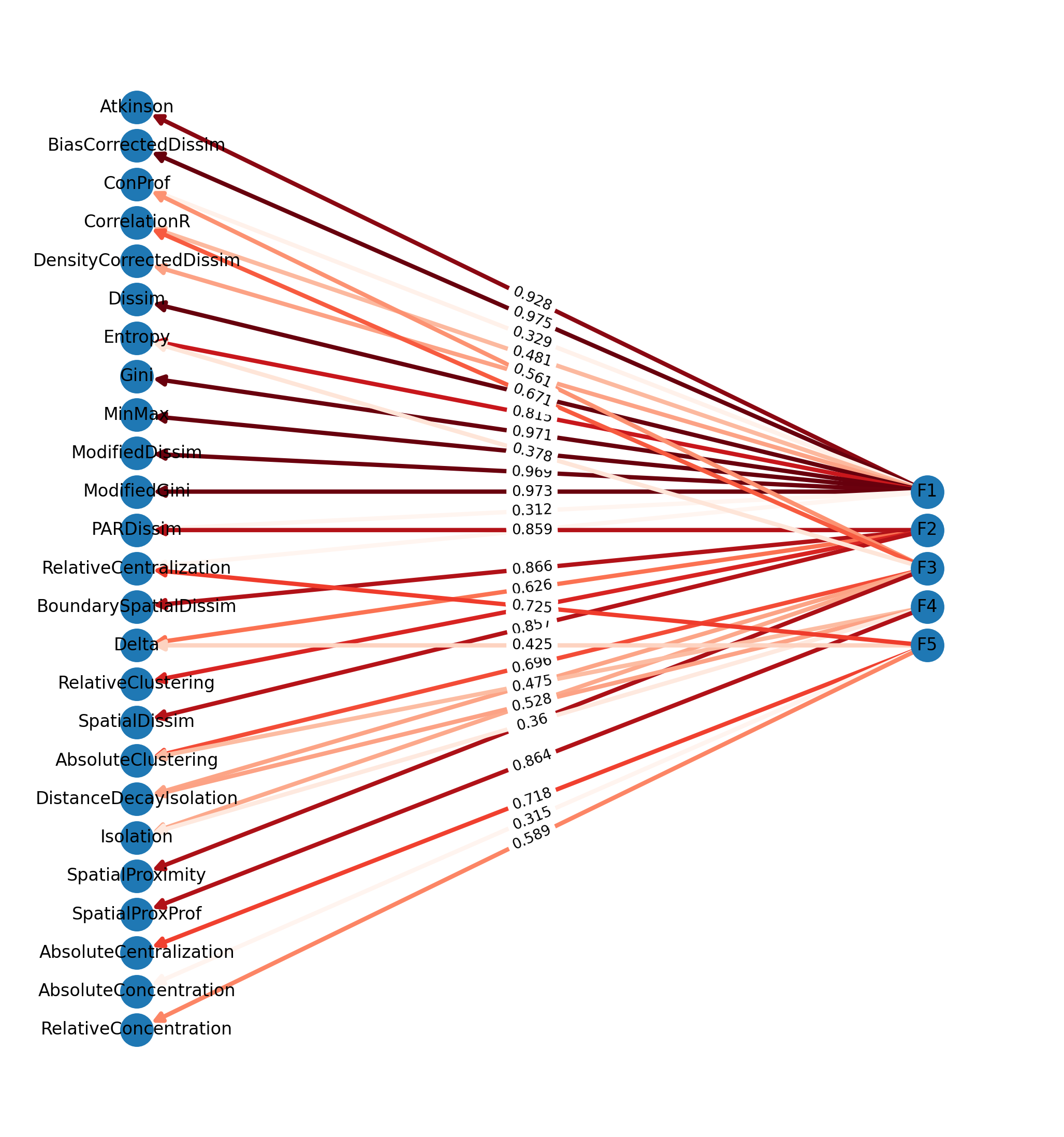
This graphic can also be done in pure networkx (i.e. without pygraphviz) using a multipartite layout, but the result isnt as nice because it doesnt group the manifest variables to avoid line crossings, and the latent variables all have the same spacing, which increases overlap

Code

f, ax = plt.subplots(figsize=(13, 14))

for layer, nodes in enumerate(reversed(tuple(nx.topological_generations(G2)))):
    # `multipartite_layout` expects the layer as a node attribute, so add the
    # numeric layer value as a node attribute
    for node in nodes:
        G2.nodes[node]["layer"] = layer

# Compute the multipartite_layout using the "layer" node attribute
pos = nx.multipartite_layout(
    G2,
    subset_key="layer",
    align="vertical",
)
nx.draw_networkx(
    G2,
    pos=pos,
    ax=ax,
    edge_cmap=plt.cm.Reds,
    edge_color=factors.T.stack().values,
    node_size=500,
    width=3,
    arrowsize=14,
)
nx.draw_networkx_edge_labels(G2, pos, edge_labels=labels)
ax.margins(0.1, None)  # add some horizontal space to fit labels
ax.axis('off')

(-0.027222222222222224,
 0.08277777777777777,
 -1.2100000000000002,
 1.2100000000000002)

21.3 Multi-Group Measures

Following

Code

if not os.path.exists(f"../data/multigroup_measures.csv"):
    dfs = []
    for metro in msa_fips:
        try:
            df = gio.get_acs(datasets, msa_fips=metro, level="bg", years=[2021])
            df = df.dropna(subset=["geometry"]).to_crs(df.estimate_utm_crs())
            seg = batch_compute_multigroup(df, groups=multi_groups, distance=2000)
            dfs.append(seg.Statistic.rename(metro))
        except Exception as e:  # PR will fail
            print(e)
            df = None
            pass
    results = pd.concat(dfs, axis=1).T
    results.to_csv(f"../data/multigroup_measures.csv")

Code

results_multi = pd.read_csv("../data/multigroup_measures.csv", index_col=0)

Code

results_multi

	GlobalDistortion	MultiDissim	MultiDivergence	MultiDiversity	MultiGini	MultiInfoTheory	MultiNormExposure	MultiRelativeDiversity	MultiSquaredCoefVar	SimpsonsConcentration	SimpsonsInteraction
10180	3.0591	0.2673	0.0827	0.9546	0.3718	0.0867	0.0894	0.0847	0.0570	0.4510	0.5490
10420	17.1550	0.4556	0.1575	0.7908	0.6000	0.1992	0.2183	0.2032	0.1079	0.5714	0.4286
10500	6.0888	0.5272	0.2333	0.8154	0.6913	0.2861	0.3310	0.3163	0.1514	0.5043	0.4957
10540	0.7949	0.2326	0.0314	0.4983	0.3146	0.0630	0.0384	0.0369	0.0194	0.7323	0.2677
10580	14.5605	0.3502	0.1169	0.9452	0.4758	0.1236	0.1384	0.1170	0.0726	0.5073	0.4927
...	...	...	...	...	...	...	...	...	...	...	...
49420	8.1606	0.4097	0.1384	0.8083	0.5436	0.1713	0.2149	0.2098	0.0891	0.4848	0.5152
49620	10.1244	0.4475	0.1525	0.9006	0.5436	0.1694	0.1945	0.1630	0.0899	0.5057	0.4943
49660	12.2645	0.5026	0.1643	0.6844	0.6598	0.2400	0.2562	0.2309	0.1201	0.6336	0.3664
49700	2.2137	0.2239	0.0788	1.0918	0.3186	0.0721	0.0652	0.0652	0.0552	0.3738	0.6262
49740	8.5083	0.3735	0.1387	0.7294	0.5491	0.1901	0.2086	0.2006	0.0832	0.5565	0.4435

384 rows × 11 columns

Code

sns.clustermap(
    results_multi.corr(), cmap="RdBu_r", annot=True, fmt=".2f", figsize=(10, 10)
)

Code

# first look for n_factors)
famulti = FactorAnalyzer(rotation="oblimin", n_factors=results_multi.shape[1])

Code

famulti.fit(results_multi.fillna(0))

FactorAnalyzer(n_factors=11, rotation='oblimin', rotation_kwargs={})

Code

ev, v = famulti.get_eigenvalues()

Code

ev = pd.Series(ev)

Code

ev.iloc[:10].plot(grid=True, style=".-")

Code

apmulti = AffinityPropagation().fit_predict(results_multi.corr())

Code

apmulti = pd.Series(dict(zip(results_multi.columns.values, apmulti)), name="Index Type")

Code

apmulti.nunique()

Code

silhouette_score(results_multi.corr(), apmulti)

0.604091489960529

Code

apmulti.sort_values()

GlobalDistortion          0
MultiDiversity            1
SimpsonsInteraction       1
MultiDissim               2
MultiDivergence           2
MultiGini                 2
MultiInfoTheory           2
MultiNormExposure         2
MultiRelativeDiversity    2
MultiSquaredCoefVar       2
SimpsonsConcentration     3
Name: Index Type, dtype: int64

:::